SwinTransformer解读
文档摘要
Swin Transformer解读 [Swin-T] Swin Transformer: Hierarchical Vision Transformer using Shifted Windows Ze Liu, Yutong Lin, Yue Cao, Han Hu, Yixuan Wei, Zheng Zhang, Stephen Lin, Baining Guo. ICCV 2021.
Swin Transformer解读
[Swin-T] Swin Transformer: Hierarchical Vision Transformer using Shifted Windows
Ze Liu, Yutong Lin, Yue Cao, Han Hu, Yixuan Wei, Zheng Zhang, Stephen Lin, Baining Guo.
ICCV 2021. [paper] [code]
解读者:沈豪,复旦大学博士,Datawhale成员
前言
《Swin Transformer: Hierarchical Vision Transformer using Shifted Windows》作为2021 ICCV最佳论文,屠榜了各大CV任务,性能优于DeiT、ViT和EfficientNet等主干网络,已经替代经典的CNN架构,成为了计算机视觉领域通用的backbone。它基于了ViT模型的思想,创新性的引入了滑动窗口机制,让模型能够学习到跨窗口的信息,同时也。同时通过下采样层,使得模型能够处理超分辨率的图片,节省计算量以及能够关注全局和局部的信息。而本文将从原理和代码角度详细解析Swin Transformer的架构。
目前将 Transformer 从自然语言处理领域应用到计算机视觉领域主要有两大挑战:
- 视觉实体的方差较大,例如同一个物体,拍摄角度不同,转化为二进制后的图片就会具有很大的差异。同时在不同场景下视觉 Transformer 性能未必很好。
- 图像分辨率高,像素点多,如果采用ViT模型,自注意力的计算量会与像素的平方成正比。
针对上述两个问题,论文中提出了一种基于滑动窗口机制,具有层级设计(下采样层) 的 Swin Transformer。
其中滑窗操作包括不重叠的 local window,和重叠的 cross-window。将注意力计算限制在一个窗口(window size固定)中,一方面能引入 CNN 卷积操作的局部性,另一方面能大幅度节省计算量,它只和窗口数量成线性关系。通过下采样的层级设计,能够逐渐增大感受野,从而使得注意力机制也能够注意到全局的特征。
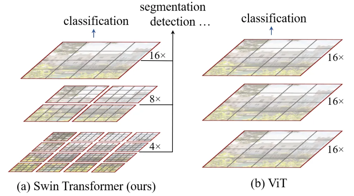
在论文的最后,作者也通过大量的实验证明Swin Transformer相较于以前的SOTA模型均有提高,尤其是在ADE20K数据和COCO数据集上的表现。也证明了Swin Transformer可以作为一种通用骨干网络被使用。
模型结构
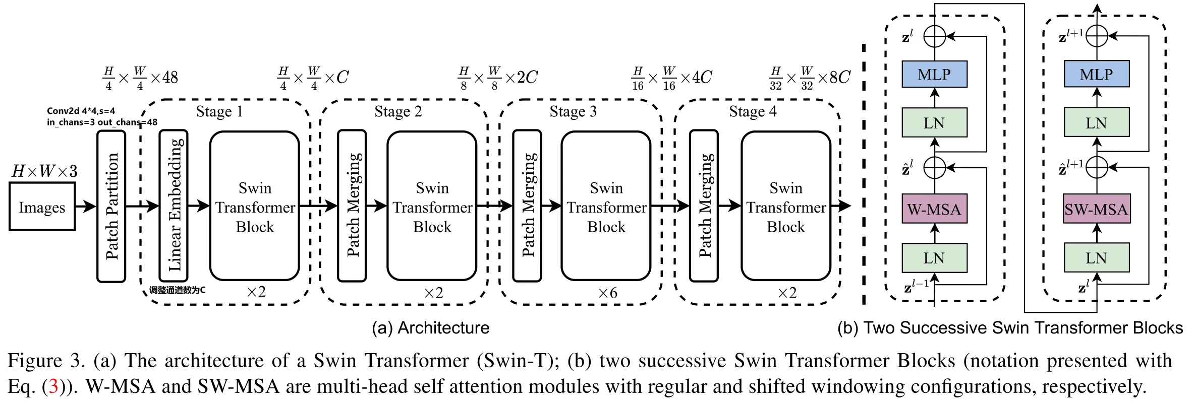
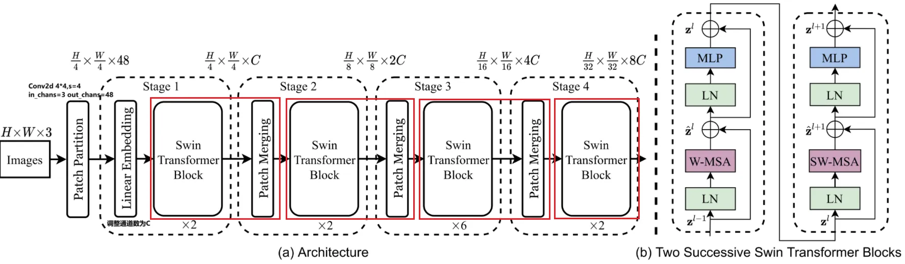
整个模型采取层次化的设计,一共包含 4 个 Stage,除第一个 stage 外,每个 stage 都会先通过 Patch Merging 层缩小输入特征图的分辨率,进行下采样操作,像 CNN 一样逐层扩大感受野,以便获取到全局的信息。
以论文的角度:
- 在输入开始的时候,做了一个
Patch Partition,即ViT中Patch Embedding操作,通过 Patch_size 为4的卷积层将图片切成一个个 Patch ,并嵌入到Embedding,将 embedding_size 转变为48(可以将 CV 中图片的通道数理解为NLP中token的词嵌入长度)。 - 随后在第一个Stage中,通过
Linear Embedding调整通道数为C。 - 在每个 Stage 里(除第一个 Stage ),均由
Patch Merging和多个Swin Transformer Block组成。 - 其中
Patch Merging模块主要在每个 Stage 一开始降低图片分辨率,进行下采样的操作。 - 而
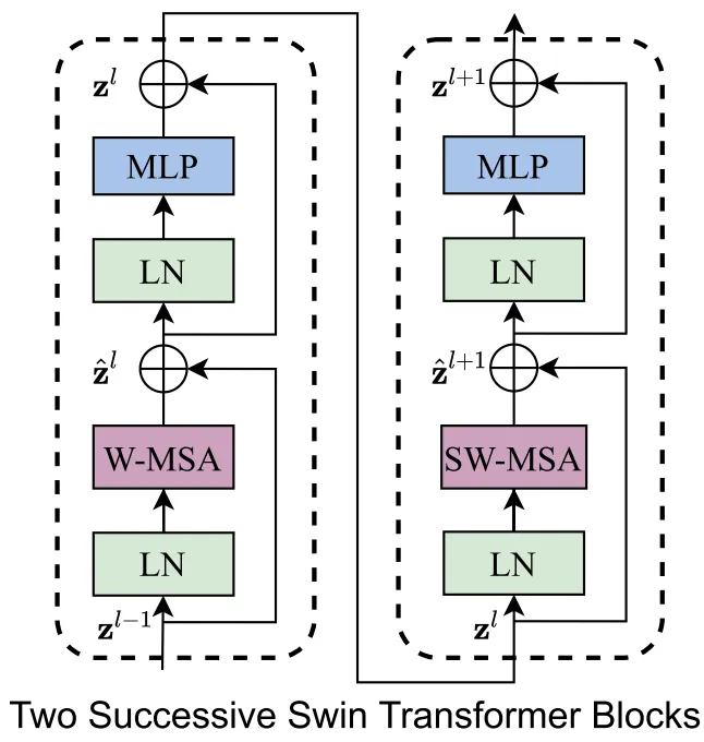
Swin Transformer Block具体结构如右图所示,主要是LayerNorm,Window Attention,Shifted Window Attention和MLP组成 。
从代码的角度:
在微软亚洲研究院提供的代码中,是将Patch Merging作为每个 Stage 最后结束的操作,输入先进行Swin Transformer Block操作,再下采样。而最后一个 Stage 不需要进行下采样操作,之间通过后续的全连接层与 target label 计算损失。
# window_size=7 # input_batch_image.shape=[128,3,224,224] class SwinTransformer(nn.Module): def __init__(...): super().__init__() ... # absolute position embedding if self.ape: self.absolute_pos_embed = nn.Parameter(torch.zeros(1, num_patches, embed_dim)) self.pos_drop = nn.Dropout(p=drop_rate) # build layers self.layers = nn.ModuleList() for i_layer in range(self.num_layers): layer = BasicLayer(...) self.layers.append(layer) self.norm = norm_layer(self.num_features) self.avgpool = nn.AdaptiveAvgPool1d(1) self.head = nn.Linear(self.num_features, num_classes) if num_classes > 0 else nn.Identity() def forward_features(self, x): x = self.patch_embed(x) # Patch Partition if self.ape: x = x + self.absolute_pos_embed x = self.pos_drop(x) for layer in self.layers: x = layer(x) x = self.norm(x) # Batch_size Windows_num Channels x = self.avgpool(x.transpose(1, 2)) # Batch_size Channels 1 x = torch.flatten(x, 1) return x def forward(self, x): x = self.forward_features(x) x = self.head(x) # self.head => Linear(in=Channels,out=Classification_num) return x
其中有几个地方处理方法与 ViT 不同:
- ViT 在输入会给 embedding 进行位置编码。而 Swin-T 这里则是作为一个可选项(
self.ape),Swin-T 是在计算 Attention 的时候做了一个相对位置编码,我认为这是这篇论文设计最巧妙的地方。 - ViT 会单独加上一个可学习参数,作为分类的 token。而 Swin-T 则是直接做平均(avgpool),输出分类,有点类似 CNN 最后的全局平均池化层。
Patch Embedding
在输入进 Block 前,我们需要将图片切成一个个 patch,然后嵌入向量。
具体做法是对原始图片裁成一个个 window_size * window_size 的窗口大小,然后进行嵌入。
这里可以通过二维卷积层,将 stride,kernel_size 设置为 window_size 大小。设定输出通道来确定嵌入向量的大小。最后将 H,W 维度展开,并移动到第一维度。
论文中输出通道设置为48,但是代码中为96,以下我们均以代码为准。
Batch_size=128

import torch import torch.nn as nn class PatchEmbed(nn.Module): def __init__(self, img_size=224, patch_size=4, in_chans=3, embed_dim=96, norm_layer=None): super().__init__() img_size = to_2tuple(img_size) # -> (img_size, img_size) patch_size = to_2tuple(patch_size) # -> (patch_size, patch_size) patches_resolution = [img_size[0] // patch_size[0], img_size[1] // patch_size[1]] self.img_size = img_size self.patch_size = patch_size self.patches_resolution = patches_resolution self.num_patches = patches_resolution[0] * patches_resolution[1] self.in_chans = in_chans self.embed_dim = embed_dim self.proj = nn.Conv2d(in_chans, embed_dim, kernel_size=patch_size, stride=patch_size) if norm_layer is not None: self.norm = norm_layer(embed_dim) else: self.norm = None def forward(self, x): # 假设采取默认参数,论文中embedding_size是96,但是代码中为48.我们以代码为准 x = self.proj(x) # 出来的是(N, 96, 224/4, 224/4) x = torch.flatten(x, 2) # 把HW维展开,(N, 96, 56*56) x = torch.transpose(x, 1, 2) # 把通道维放到最后 (N, 56*56, 96) if self.norm is not None: x = self.norm(x) return x
Patch Merging
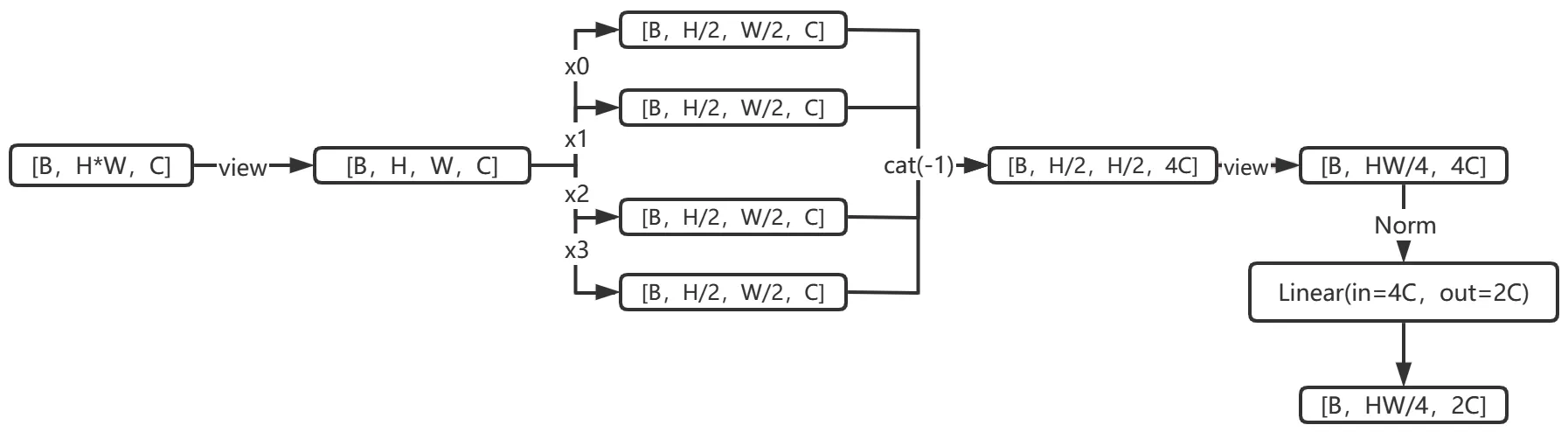
该模块的作用是在每个 Stage 开始前做降采样,用于缩小分辨率,调整通道数进而形成层次化的设计,同时也能节省一定运算量。
在 CNN 中,则是在每个 Stage 开始前用
stride=2的卷积/池化层来降低分辨率。
每次降采样是两倍,因此在行方向和列方向上,间隔 2 选取元素。
然后拼接在一起作为一整个张量,最后展开。此时通道维度会变成原先的 4 倍(因为 H,W 各缩小 2 倍),此时再通过一个全连接层再调整通道维度为原来的两倍。
下面是一个示意图(输入张量 N=1, H=W=8, C=1,不包含最后的全连接层调整)

class PatchMerging(nn.Module): def __init__(self, input_resolution, dim, norm_layer=nn.LayerNorm): super().__init__() self.input_resolution = input_resolution self.dim = dim self.reduction = nn.Linear(4 * dim, 2 * dim, bias=False) self.norm = norm_layer(4 * dim) def forward(self, x): """ x: B, H*W, C """ H, W = self.input_resolution B, L, C = x.shape assert L == H * W, "input feature has wrong size" assert H % 2 == 0 and W % 2 == 0, f"x size ({H}*{W}) are not even." x = x.view(B, H, W, C) x0 = x[:, 0::2, 0::2, :] # B H/2 W/2 C x1 = x[:, 1::2, 0::2, :] # B H/2 W/2 C x2 = x[:, 0::2, 1::2, :] # B H/2 W/2 C x3 = x[:, 1::2, 1::2, :] # B H/2 W/2 C x = torch.cat([x0, x1, x2, x3], -1) # B H/2 W/2 4*C x = x.view(B, -1, 4 * C) # B H/2*W/2 4*C x = self.norm(x) x = self.reduction(x) return x
Window Partition/Reverse
window partition函数是用于对张量划分窗口,指定窗口大小。将原本的张量从 N H W C, 划分成 num_windows*B, window_size, window_size, C,其中 num_windows = H*W / window_size*window_size,即窗口的个数。而window reverse函数则是对应的逆过程。这两个函数会在后面的Window Attention用到。
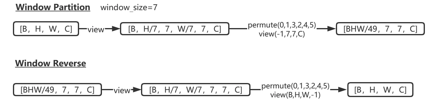
def window_partition(x, window_size): B, H, W, C = x.shape x = x.view(B, H // window_size, window_size, W // window_size, window_size, C) windows = x.permute(0, 1, 3, 2, 4, 5).contiguous().view(-1, window_size, window_size, C) return windows def window_reverse(windows, window_size, H, W): B = int(windows.shape[0] / (H * W / window_size / window_size)) x = windows.view(B, H // window_size, W // window_size, window_size, window_size, -1) x = x.permute(0, 1, 3, 2, 4, 5).contiguous().view(B, H, W, -1) return x
Window Attention
传统的 Transformer 都是基于全局来计算注意力的,因此计算复杂度十分高。而 Swin Transformer 则将注意力的计算限制在每个窗口内,进而减少了计算量。我们先简单看下公式
主要区别是在原始计算 Attention 的公式中的 Q,K 时加入了相对位置编码。
class WindowAttention(nn.Module): r""" Window based multi-head self attention (W-MSA) module with relative position bias. It supports both of shifted and non-shifted window. Args: dim (int): Number of input channels. window_size (tuple[int]): The height and width of the window. num_heads (int): Number of attention heads. qkv_bias (bool, optional): If True, add a learnable bias to query, key, value. Default: True qk_scale (float | None, optional): Override default qk scale of head_dim ** -0.5 if set attn_drop (float, optional): Dropout ratio of attention weight. Default: 0.0 proj_drop (float, optional): Dropout ratio of output. Default: 0.0 """ def __init__(self, dim, window_size, num_heads, qkv_bias=True, qk_scale=None, attn_drop=0., proj_drop=0.): super().__init__() self.dim = dim self.window_size = window_size # Wh, Ww self.num_heads = num_heads # nH head_dim = dim // num_heads # 每个注意力头对应的通道数 self.scale = qk_scale or head_dim ** -0.5 # define a parameter table of relative position bias self.relative_position_bias_table = nn.Parameter( torch.zeros((2 * window_size[0] - 1) * (2 * window_size[1] - 1), num_heads)) # 设置一个形状为(2*(Wh-1) * 2*(Ww-1), nH)的可学习变量,用于后续的位置编码 self.qkv = nn.Linear(dim, dim * 3, bias=qkv_bias) self.attn_drop = nn.Dropout(attn_drop) self.proj = nn.Linear(dim, dim) self.proj_drop = nn.Dropout(proj_drop) trunc_normal_(self.relative_position_bias_table, std=.02) self.softmax = nn.Softmax(dim=-1) # 相关位置编码...
相关位置编码的直观理解
Q,K,V.shape=[numWindwos*B, num_heads, window_size*window_size, head_dim]
- window_size*window_size 即 NLP 中
token的个数- head\_dim=\frac{Embedding\_dim}{num\_heads} 即 NLP 中
token的词嵌入向量的维度{QK}^T计算出来的
Attention张量的形状为[numWindows*B, num_heads, Q_tokens, K_tokens]
- 其中Q_tokens=K_tokens=window_size*window_size
以window_size=2为例:
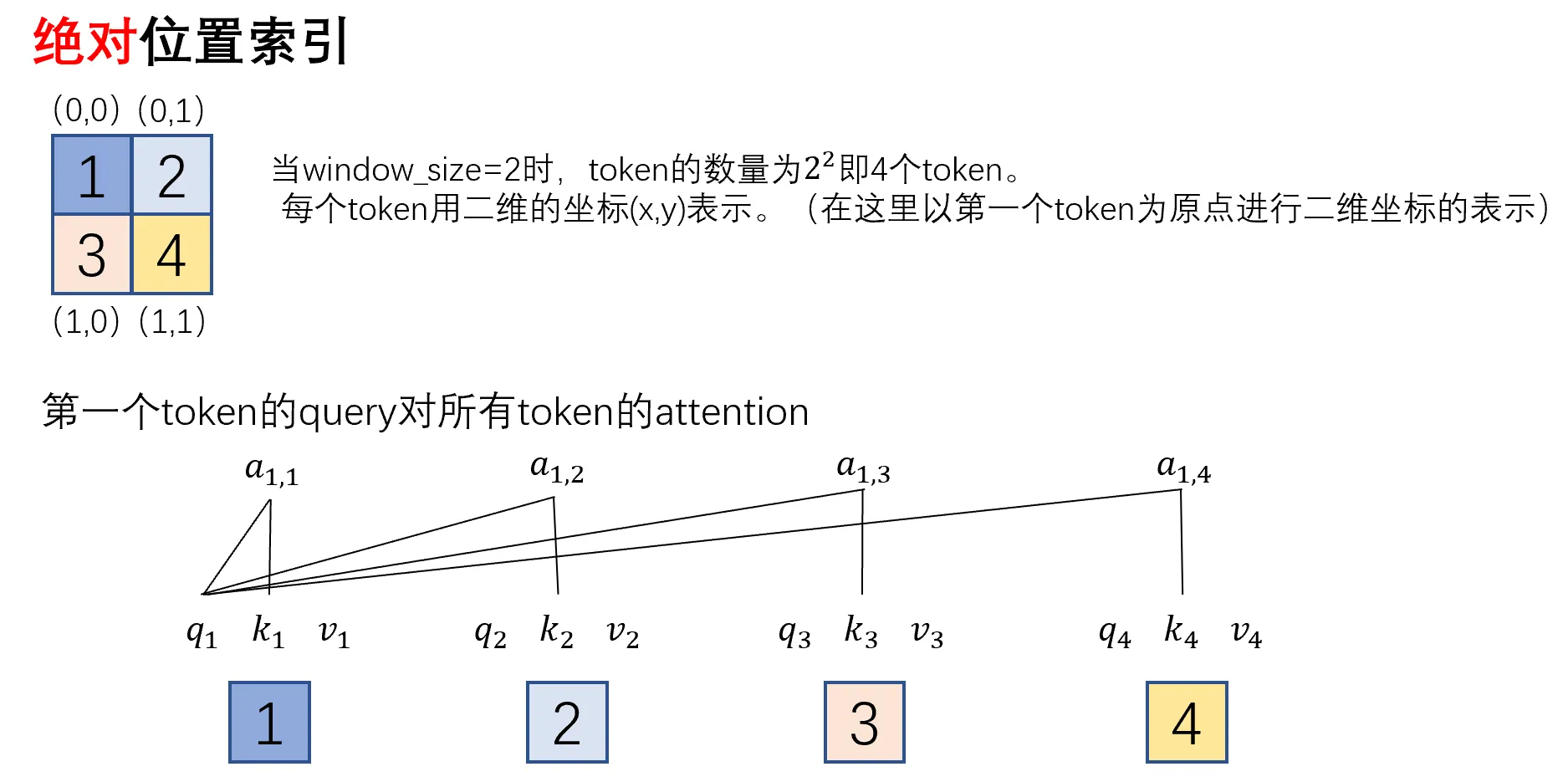
因此:{QK}^T=\left[\begin{array}{cccc}a_{11} & a_{12} & a_{13} & a_{14} \\ a_{21} & a_{22} & a_{23} & a_{24} \\ a_{31} & a_{32} & a_{33} & a_{34} \\ a_{41} & a_{42} & a_{43} & a_{44}\end{array}\right]
- 第 i 行表示第 i 个 token 的
query对所有token的key的attention。 - 对于 Attention 张量来说,以不同元素为原点,其他元素的坐标也是不同的,
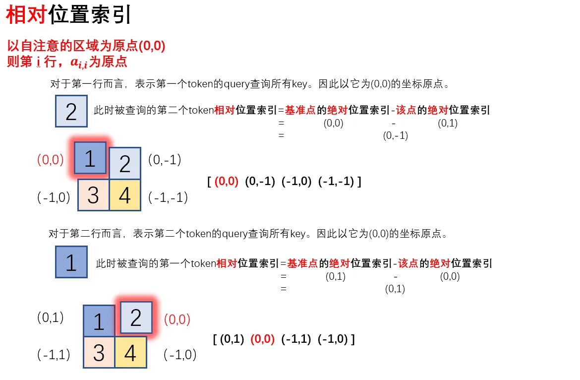
所以{QK}^T的相对位置索引=\left[\begin{array}{cccc}(0,0) & (0,-1) & (-1,0) & (-1,-1) \\ (0,1) & (0,0) & (-1,1) & (-1,0) \\ (1,0) & (1,-1) & (0,0) & (0,-1) \\ (1,1) & (1,0) & (0,1) & (0,0)\end{array}\right]
由于最终我们希望使用一维的位置坐标 x+y 代替二维的位置坐标 (x,y),为了避免 (1,2) (2,1) 两个坐标转为一维时均为3,我们之后对相对位置索引进行了一些线性变换,使得能通过一维的位置坐标唯一映射到一个二维的位置坐标,详细可以通过代码部分进行理解。
相关位置编码的代码详解
首先我们利用torch.arange和torch.meshgrid函数生成对应的坐标,这里我们以windowsize=2为例子
coords_h = torch.arange(self.window_size[0]) coords_w = torch.arange(self.window_size[1]) coords = torch.meshgrid([coords_h, coords_w]) # -> 2*(wh, ww) """ (tensor([[0, 0], [1, 1]]), tensor([[0, 1], [0, 1]])) """
然后堆叠起来,展开为一个二维向量
coords = torch.stack(coords) # 2, Wh, Ww coords_flatten = torch.flatten(coords, 1) # 2, Wh*Ww """ tensor([[0, 0, 1, 1], [0, 1, 0, 1]]) """
利用广播机制,分别在第一维,第二维,插入一个维度,进行广播相减,得到 2, wh*ww, wh*ww的张量
relative_coords_first = coords_flatten[:, :, None] # 2, wh*ww, 1 relative_coords_second = coords_flatten[:, None, :] # 2, 1, wh*ww relative_coords = relative_coords_first - relative_coords_second # 最终得到 2, wh*ww, wh*ww 形状的张量
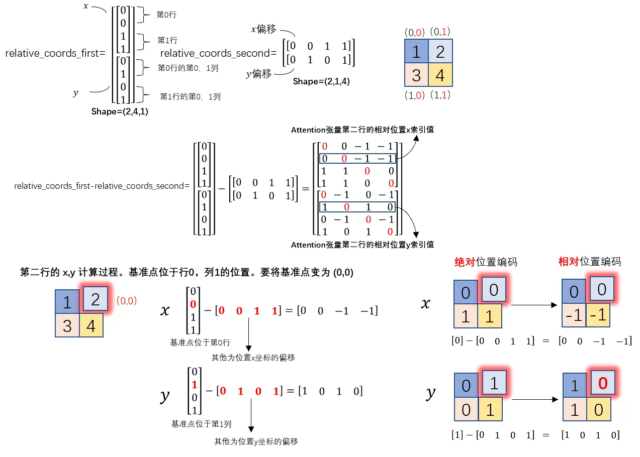
因为采取的是相减,所以得到的索引是从负数开始的,我们加上偏移量,让其从 0 开始。
relative_coords = relative_coords.permute(1, 2, 0).contiguous() # Wh*Ww, Wh*Ww, 2 relative_coords[:, :, 0] += self.window_size[0] - 1 relative_coords[:, :, 1] += self.window_size[1] - 1
后续我们需要将其展开成一维偏移量。而对于 (1,2)和(2,1)这两个坐标。在二维上是不同的,但是通过将 x,y 坐标相加转换为一维偏移的时候,他的偏移量是相等的。
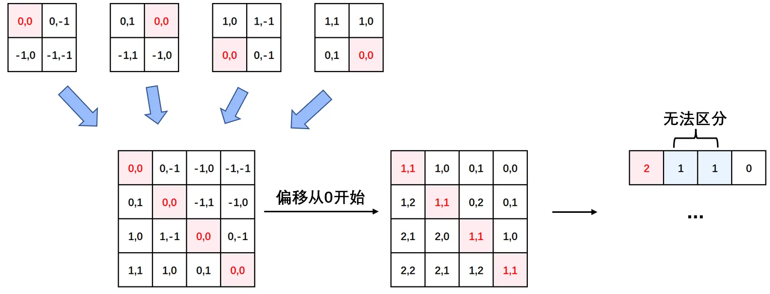
所以最后我们对其中做了个乘法操作,以进行区分
relative_coords[:, :, 0] *= 2 * self.window_size[1] - 1

然后再最后一维上进行求和,展开成一个一维坐标,并注册为一个不参与网络学习的变量
relative_position_index = relative_coords.sum(-1) # Wh*Ww, Wh*Ww self.register_buffer("relative_position_index", relative_position_index)
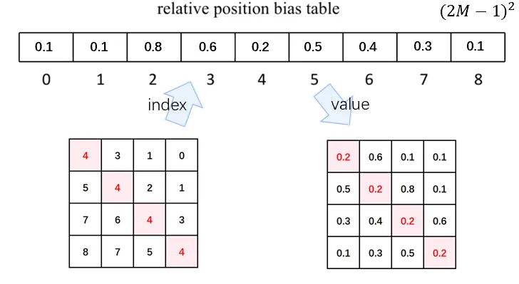
之前计算的是相对位置索引,并不是相对位置偏置参数。真正使用到的可训练参数\hat B是保存在relative position bias table表里的,这个表的长度是等于 (2M−1) × (2M−1) (在二维位置坐标中线性变化乘以2M-1导致)的。那么上述公式中的相对位置偏执参数B是根据上面的相对位置索引表根据查relative position bias table表得到的。
接着我们看前向代码
def forward(self, x, mask=None): """ Args: x: input features with shape of (num_windows*B, N, C) mask: (0/-inf) mask with shape of (num_windows, Wh*Ww, Wh*Ww) or None """ B_, N, C = x.shape qkv = self.qkv(x).reshape(B_, N, 3, self.num_heads, C // self.num_heads).permute(2, 0, 3, 1, 4) q, k, v = qkv[0], qkv[1], qkv[2] # make torchscript happy (cannot use tensor as tuple) q = q * self.scale attn = (q @ k.transpose(-2, -1)) relative_position_bias = self.relative_position_bias_table[self.relative_position_index.view(-1)].view(self.window_size[0] * self.window_size[1], self.window_size[0] * self.window_size[1], -1) # Wh*Ww,Wh*Ww,nH relative_position_bias = relative_position_bias.permute(2, 0, 1).contiguous() # nH, Wh*Ww, Wh*Ww attn = attn + relative_position_bias.unsqueeze(0) # (1, num_heads, windowsize, windowsize) if mask is not None: # 下文会分析到 ... else: attn = self.softmax(attn) attn = self.attn_drop(attn) x = (attn @ v).transpose(1, 2).reshape(B_, N, C) x = self.proj(x) x = self.proj_drop(x) return x
- 首先输入张量形状为
[numWindows*B, window_size * window_size, C] - 然后经过
self.qkv这个全连接层后,进行 reshape,调整轴的顺序,得到形状为[3, numWindows*B, num_heads, window_size*window_size, c//num_heads],并分配给q,k,v。 - 根据公式,我们对
q乘以一个scale缩放系数,然后与k(为了满足矩阵乘要求,需要将最后两个维度调换)进行相乘。得到形状为[numWindows*B, num_heads, window_size*window_size, window_size*window_size]的attn张量 - 之前我们针对位置编码设置了个形状为
(2*window_size-1*2*window_size-1, numHeads)的可学习变量。我们用计算得到的相对编码位置索引self.relative_position_index.vew(-1)选取,得到形状为(window_size*window_size, window_size*window_size, numHeads)的编码,再permute(2,0,1)后加到attn张量上 - 暂不考虑 mask 的情况,剩下就是跟 transformer 一样的 softmax,dropout,与
V矩阵乘,再经过一层全连接层和 dropout
Shifted Window Attention
前面的 Window Attention 是在每个窗口下计算注意力的,为了更好的和其他 window 进行信息交互,Swin Transformer 还引入了 shifted window 操作。
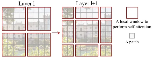
左边是没有重叠的 Window Attention,而右边则是将窗口进行移位的 Shift Window Attention。可以看到移位后的窗口包含了原本相邻窗口的元素。但这也引入了一个新问题,即 window 的个数翻倍了,由原本四个窗口变成了 9 个窗口。在实际代码里,我们是通过对特征图移位,并给 Attention 设置 mask 来间接实现的。能在保持原有的 window 个数下,最后的计算结果等价。
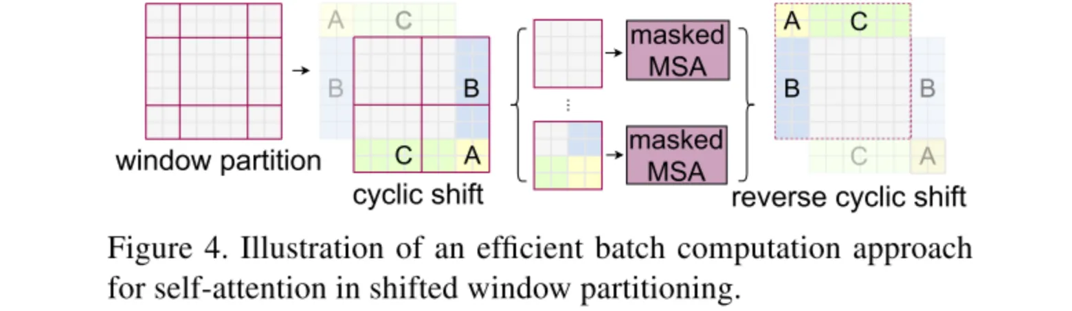
特征图移位操作
代码里对特征图移位是通过torch.roll来实现的,下面是示意图
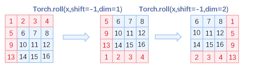
如果需要
reverse cyclic shift的话只需把参数shifts设置为对应的正数值。
Attention Mask
这是 Swin Transformer 的精华,通过设置合理的 mask,让Shifted Window Attention在与Window Attention相同的窗口个数下,达到等价的计算结果。
首先我们对 Shift Window 后的每个窗口都给上 index,并且做一个roll操作(window_size=2, shift_size=1)
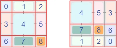
我们希望在计算 Attention 的时候,让具有相同 index QK 进行计算,而忽略不同 index QK 计算结果。最后正确的结果如下图所示
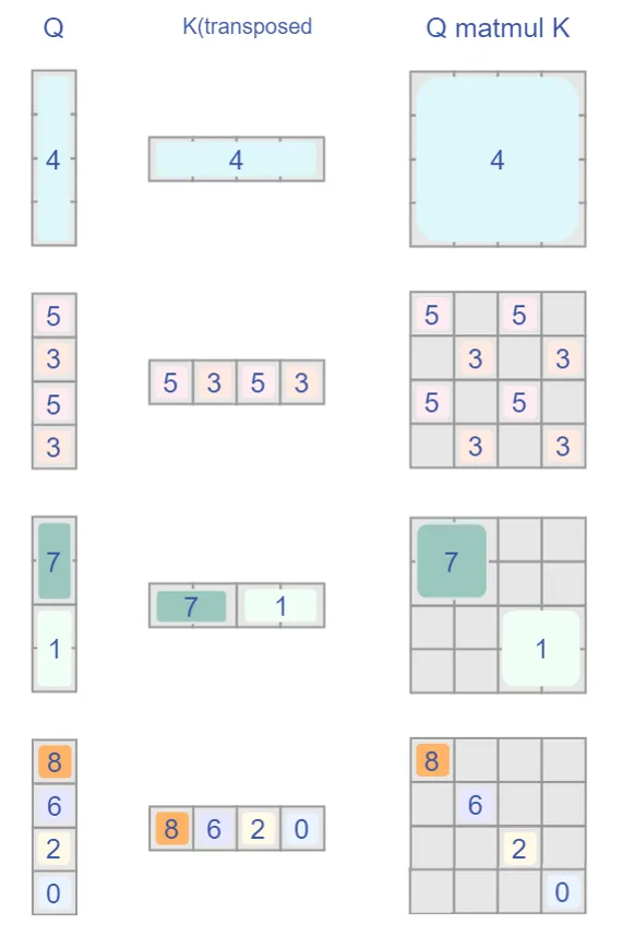
而要想在原始四个窗口下得到正确的结果,我们就必须给 Attention 的结果加入一个 mask(如上图最右边所示)相关代码如下:
if self.shift_size > 0: # calculate attention mask for SW-MSA H, W = self.input_resolution img_mask = torch.zeros((1, H, W, 1)) # 1 H W 1 h_slices = (slice(0, -self.window_size), slice(-self.window_size, -self.shift_size), slice(-self.shift_size, None)) w_slices = (slice(0, -self.window_size), slice(-self.window_size, -self.shift_size), slice(-self.shift_size, None)) cnt = 0 for h in h_slices: for w in w_slices: img_mask[:, h, w, :] = cnt cnt += 1 mask_windows = window_partition(img_mask, self.window_size) # nW, window_size, window_size, 1 mask_windows = mask_windows.view(-1, self.window_size * self.window_size) attn_mask = mask_windows.unsqueeze(1) - mask_windows.unsqueeze(2) attn_mask = attn_mask.masked_fill(attn_mask != 0, float(-100.0)).masked_fill(attn_mask == 0, float(0.0)) else: attn_mask = None
以上图的设置,我们用这段代码会得到这样的一个 mask
tensor([[[[[ 0., 0., 0., 0.], [ 0., 0., 0., 0.], [ 0., 0., 0., 0.], [ 0., 0., 0., 0.]]], [[[ 0., -100., 0., -100.], [-100., 0., -100., 0.], [ 0., -100., 0., -100.], [-100., 0., -100., 0.]]], [[[ 0., 0., -100., -100.], [ 0., 0., -100., -100.], [-100., -100., 0., 0.], [-100., -100., 0., 0.]]], [[[ 0., -100., -100., -100.], [-100., 0., -100., -100.], [-100., -100., 0., -100.], [-100., -100., -100., 0.]]]]])
在之前的 window attention 模块的前向代码里,包含这么一段
if mask is not None: nW = mask.shape[0] # 一张图被分为多少个windows eg:[4,49,49] attn = attn.view(B_ // nW, nW, self.num_heads, N, N) + mask.unsqueeze(1).unsqueeze(0) # torch.Size([128, 4, 12, 49, 49]) torch.Size([1, 4, 1, 49, 49]) attn = attn.view(-1, self.num_heads, N, N) attn = self.softmax(attn) else: attn = self.softmax(attn)
将 mask 加到 attention 的计算结果,并进行 softmax。mask 的值设置为 - 100,softmax 后就会忽略掉对应的值。关于Mask,我们发现在官方代码库中的issue38也进行了讨论:-->The Question about the mask of window attention #38
W-MSA和MSA的复杂度对比
在原论文中,作者提出的基于滑动窗口操作的 W-MSA 能大幅度减少计算量。那么两者的计算量和算法复杂度大概是如何的呢,论文中给出了一下两个公式进行对比。
- h:feature map的高度
- w:feature map的宽度
- C:feature map的通道数(也可以称为embedding size的大小)
- M:window_size的大小
MSA模块的计算量
首先对于feature map中每一个token(一共有 hw 个token,通道数为C),记作X^{h w \times C},需要通过三次线性变换 W_q,W_k,W_v ,产生对应的q,k,v向量,记作 Q^{h w \times C},K^{h w \times C},V^{h w \times C} (通道数为C)。
根据矩阵运算的计算量公式可以得到运算量为 3hwC \times C ,即为 3hwC^2 。
忽略除以\sqrt d 以及softmax的计算量,根据根据矩阵运算的计算量公式可得 hwC \times hw + hw^2 \times C ,即为 2(hw^2)C 。
最终再通过一个Linear层输出,计算量为 hwC^2 。因此整体的计算量为 4 h w C^{2}+2(h w)^{2} C 。
W-MSA模块的计算量
对于W-MSA模块,首先会将feature map根据window_size分成 \frac{hw}{M^2} 的窗口,每个窗口的宽高均为M,然后在每个窗口进行MSA的运算。因此,可以利用上面MSA的计算量公式,将 h=M,w=M 带入,可以得到一个窗口的计算量为 4 M^2 C^{2}+2M^{4} C 。
又因为有 \frac{hw}{M^2} 个窗口,则:
假设feature map的h=w=112,M=7,C=128,采用W-MSA模块会比MSA模块节省约40124743680 FLOPs:
整体流程图
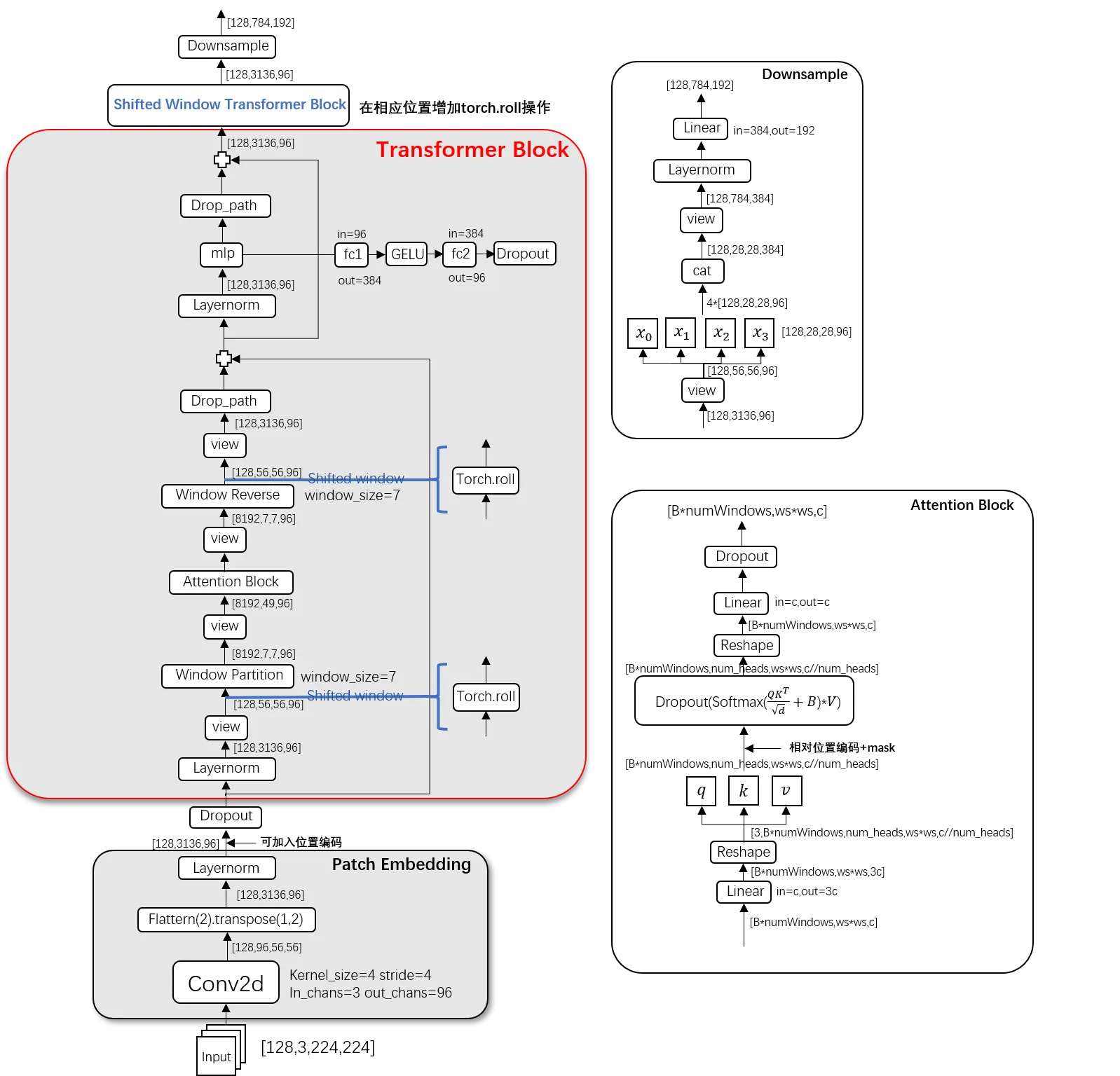
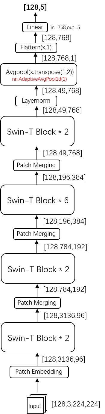
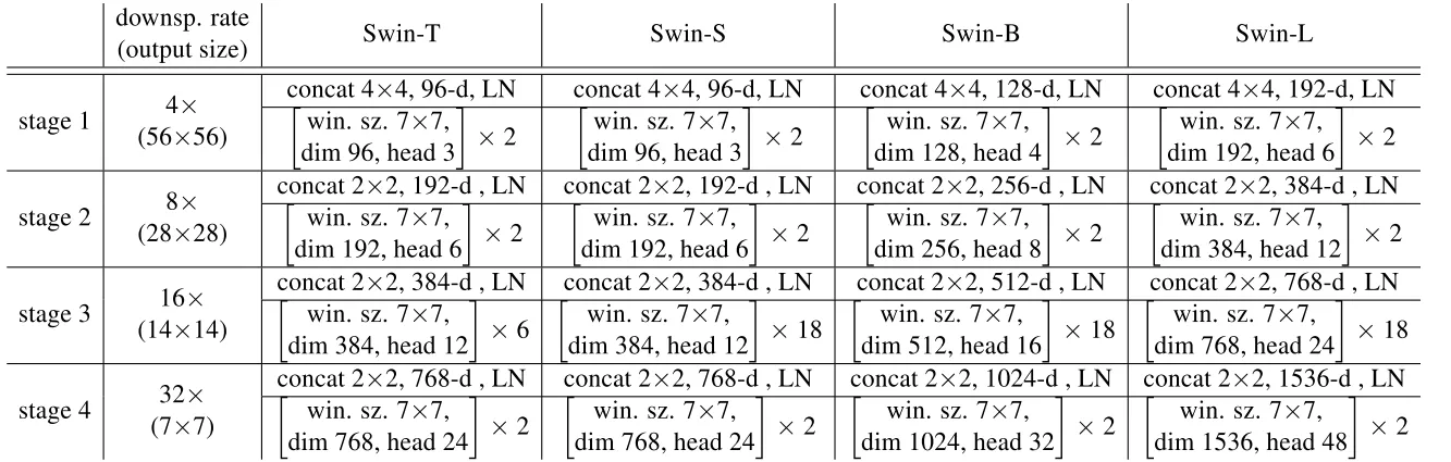
参考博客:
联系方式: