HNSW算法
文档摘要
HNSW算法 1.HNSW的灵感来源:两大核心思想 HNSW的成功,源于它巧妙地结合了两种经典的思想: 1.小世界网络:大家可能听过“六度分隔理论”,意思是地球上任何两个人,平均只需要通过六个中间人就能建立起联系。这就是小世界网络的体现 。这种网络的特点是: 高聚类性:你的朋友之间,彼此也很可能互相是朋友(形成聚集的小团体)。 短平均路径:尽管有聚集性,但任意两个节点之间的平均距离却很短。HNSW的目标就是构建一个具有类似特性的图,使得可以从任意节点出发,用很少的“步数”(跳跃)到达目标节点。 2.跳表:想象一本有目录的书。目录就是书的“高层结构”,它章节标题,让你能快速定位到大概范围。然后你翻到对应章节,再通过更细的标题或页码找到具体内容。
HNSW算法
1.HNSW的灵感来源:两大核心思想
HNSW的成功,源于它巧妙地结合了两种经典的思想:
1.小世界网络:大家可能听过“六度分隔理论”,意思是地球上任何两个人,平均只需要通过六个中间人就能建立起联系。这就是小世界网络的体现
。这种网络的特点是:
- 高聚类性:你的朋友之间,彼此也很可能互相是朋友(形成聚集的小团体)。
- 短平均路径:尽管有聚集性,但任意两个节点之间的平均距离却很短。HNSW的目标就是构建一个具有类似特性的图,使得可以从任意节点出发,用很少的“步数”(跳跃)到达目标节点。
2.跳表:想象一本有目录的书。目录就是书的“高层结构”,它章节标题,让你能快速定位到大概范围。然后你翻到对应章节,再通过更细的标题或页码找到具体内容。跳表就是类似的多层索引结构,在数据链表上建立多层“快车道”,从高层粗犷检索开始,逐层细化,直到最底层找到目标,从而避免从头到尾的遍历。
HNSW正是将小世界网络的连通性和跳表的分层思想融合在了一起
2.算法原理分步详解
HNSW(Hierarchical Navigable Small World,分层可导航小世界图)是一种基于图结构的近似最近邻(ANN)搜索算法,
它通过构建一个多层次的“可导航小世界图”,让搜索过程像“在城市地图中找路”一样高效。
其核心思想是:
先在高层图中快速找到大致方向,再在底层图中精确定位目标。
下面我们来分步解析 HNSW 的工作原理。
1.图结构的构建(Index Construction)
HNSW 的核心数据结构是一个多层图(Hierarchical Graph),
每一层都是一个“小世界网络(Small World Graph)”,即节点之间存在较短的路径连接。
步骤 1:多层结构(层级随机化)
- 每个向量会被随机分配到若干层(Level 0 ~ L)。
- 层数的分布遵循指数衰减规律(高层节点少,底层节点多)。
例如:- Level 3:只有少数节点(类似城市的高速公路网)
- Level 2:节点更多(城市主干道)
- Level 1:更密集(区级道路)
- Level 0:所有节点都在这里(街道级别)
这种结构让算法能像缩放地图一样,先看宏观,再聚焦微观。
步骤 2:逐层插入节点(Layer-by-Layer Insertion)
当新向量 v 进入系统时,HNSW 会逐层插入:
-
确定插入层级
根据随机分配的层级L_v,决定v将出现在哪几层。 -
自顶向下导航
从当前最高层开始,找到与v最近的节点作为“入口点(Entry Point)”。 -
逐层下降搜索
在每一层中,执行“贪心搜索(Greedy Search)”:- 不断跳向更接近
v的邻居; - 当没有更近的节点时,停止;
- 将当前位置作为下一层的起点。
- 不断跳向更接近
-
在对应层建立连接(Linking)
在v所在的每一层,选取若干最近邻节点建立边连接(邻居数量由参数M控制)。
为保持小世界特性,HNSW 会对邻居集合进行“修剪”,确保网络稀疏且高效。
2.查询阶段(Search Process)
HNSW 的搜索过程与构建阶段类似,同样遵循“自顶向下、逐层逼近”的策略。
步骤 1:从顶层开始搜索
- 选择一个入口节点(通常是构建时的最高层入口点)。
- 在最高层使用贪心搜索找到与查询向量
q最近的节点。
步骤 2:逐层向下导航
- 将上层搜索到的最优节点作为下一层的入口;
- 在更低层的图中继续搜索,逐步缩小搜索范围;
- 每下一层,节点密度增加,搜索精度提升。
步骤 3:底层精确搜索
- 到达底层(Level 0)后,算法会使用“优先队列 + 局部扩展搜索”策略:
- 维护一个候选节点集合(Candidate List);
- 扩展其邻居并更新最近邻;
- 重复直到候选集不再变化或达到设定搜索深度(参数
ef_search)。
- 最终返回距离最近的 K 个节点。
3.关键参数说明
| 参数 | 含义 | 作用 |
|---|---|---|
M |
每个节点的最大邻居数 | 越大图越稠密,召回率高但内存开销增大 |
ef_construction |
构建阶段的搜索宽度 | 控制索引构建质量与速度 |
ef_search |
查询阶段的搜索宽度 | 值越大,精度越高但搜索时间更长 |
4.HNSW 的性能特点
- 高精度:通过层级导航逐步逼近最优解,近似结果非常接近精确搜索;
- 高效率:图结构使得搜索复杂度接近
O(log N); - 可增量更新:新节点可动态插入,无需重建索引;
- 内存友好:通过稀疏连接与层级控制,平衡性能与空间。
5. 类比理解
可以把 HNSW 想象成一场“多层地图找目标”的游戏:
| 层级 | 类比 | 搜索作用 |
|---|---|---|
| 顶层 | 全国高速公路地图 | 快速确定大致方向 |
| 中层 | 城市主干道地图 | 精确锁定区域 |
| 底层 | 街区地图 | 找到具体目标 |
在搜索过程中,算法像一个熟练的导航员,
从高速公路(高层)出发,逐层进入城区(低层),最终找到目标建筑(最邻近向量)。
✅ 总结:HNSW 的核心思想
分层导航 + 贪心搜索 + 局部连接优化
HNSW 通过在不同层次建立稀疏图结构,使搜索可以先全局定位、再局部精查,
在高维向量检索任务中实现了近似最优的性能与速度平衡。
它已成为当前向量数据库(如 Milvus、FAISS、Weaviate)中默认启用的主流索引算法。
3.HNSW算法实现
HNSW算法Python实现
3.1我们导入必要的库:
import numpy as np import random import math from collections import defaultdict import matplotlib.pyplot as plt import time from sklearn.metrics.pairwise import euclidean_distances plt.rcParams['font.sans-serif'] = ['Microsoft YaHei'] plt.rcParams['axes.unicode_minus'] = False # 设置随机种子以保证结果可重现 np.random.seed(42)
3.2实现简化的HNSW类
class SimpleHNSW: """简化的HNSW实现,用于学习演示""" def __init__(self, max_elements=1000, M=10, ef_construction=50, max_layers=6): """ 初始化HNSW索引 参数: - max_elements: 最大元素数量 - M: 每个节点的最大连接数 - ef_construction: 构建时的搜索范围 - max_layers: 最大层数 """ self.max_elements = max_elements self.M = M # 每个节点的最大连接数 self.ef_construction = ef_construction # 构建时的搜索范围 self.max_layers = max_layers # 最大层数 # 存储所有数据点 self.data_points = [] # 每层的图结构(邻接表) self.layers = [defaultdict(list) for _ in range(max_layers)] # 每个点所在的最高层 self.entry_point = None self.entry_level = -1 def _random_level(self): """随机生成节点的层级(指数分布)""" level = 0 while random.random() < 0.5 and level < self.max_layers - 1: level += 1 return level def _euclidean_distance(self, a, b): """计算欧氏距离""" return np.sqrt(np.sum((a - b) ** 2)) def _search_layer(self, query, entry_point, ef, layer): """ 在指定层搜索最近邻 """ if entry_point is None or entry_point not in self.layers[layer]: return [] visited = set([entry_point]) candidates = [(self._euclidean_distance(query, self.data_points[entry_point]), entry_point)] # 使用堆来维护候选集(这里简化为列表排序) results = [] while candidates and len(results) < ef: # 获取距离最近的候选点 candidates.sort(key=lambda x: x[0]) current_dist, current_point = candidates.pop(0) # 检查是否应该将当前点加入结果 if not results or current_dist < results[-1][0]: results.append((current_dist, current_point)) results.sort(key=lambda x: x[0]) if len(results) > ef: results = results[:ef] # 探索邻居 for neighbor in self.layers[layer][current_point]: if neighbor not in visited: visited.add(neighbor) dist = self._euclidean_distance(query, self.data_points[neighbor]) candidates.append((dist, neighbor)) return results def add_point(self, point): """向HNSW中添加新点""" if len(self.data_points) >= self.max_elements: raise ValueError("达到最大容量") point_id = len(self.data_points) self.data_points.append(point) # 确定新点的层级 level = self._random_level() # 如果是第一个点,设为入口点 if self.entry_point is None: self.entry_point = point_id self.entry_level = level for l in range(level + 1): self.layers[l][point_id] = [] # 在新点的每一层创建空邻居列表 return # 从最高层开始搜索,找到每层的最近邻 current_point = self.entry_point current_max_level = self.entry_level # 从顶层开始搜索,找到每层的入口点 for l in range(current_max_level, level, -1): if l < len(self.layers): results = self._search_layer(point, current_point, 1, l) if results: current_point = results[0][1] # 从新点的最高层开始,逐层向下插入 for l in range(min(level, current_max_level), -1, -1): # 在当前层搜索ef_construction个最近邻 results = self._search_layer(point, current_point, self.ef_construction, l) # 选择前M个最近邻作为连接 neighbors = [idx for _, idx in results[:self.M]] # 在新点的当前层创建连接 self.layers[l][point_id] = neighbors.copy() # 双向连接:邻居也连接到新点 for neighbor in neighbors: if len(self.layers[l][neighbor]) < self.M: self.layers[l][neighbor].append(point_id) else: # 如果邻居连接数已满,替换最远的连接 neighbor_neighbors = self.layers[l][neighbor] distances = [self._euclidean_distance(self.data_points[neighbor], self.data_points[n]) for n in neighbor_neighbors] max_idx = np.argmax(distances) if self._euclidean_distance(self.data_points[neighbor], point) < distances[max_idx]: neighbor_neighbors[max_idx] = point_id # 更新当前点用于下一层 if results: current_point = results[0][1] # 如果新点的层级比当前入口点高,更新入口点 if level > self.entry_level: self.entry_point = point_id self.entry_level = level def search(self, query, k=5, ef_search=50): """在HNSW中搜索最近邻""" if self.entry_point is None: return [] current_point = self.entry_point current_level = self.entry_level # 从顶层开始搜索 for l in range(current_level, 0, -1): results = self._search_layer(query, current_point, 1, l) if results: current_point = results[0][1] # 在最底层进行精细搜索 results = self._search_layer(query, current_point, ef_search, 0) # 返回前k个结果 return [(idx, dist) for dist, idx in results[:k]]
3.3第三步:生成示例数据和可视化函数
def generate_sample_data(n_samples=200, dim=2): """生成示例数据:四个分离的高斯分布簇""" clusters = [] # 创建四个簇 cluster1 = np.random.normal(loc=[2, 2], scale=0.3, size=(n_samples//4, dim)) cluster2 = np.random.normal(loc=[8, 3], scale=0.4, size=(n_samples//4, dim)) cluster3 = np.random.normal(loc=[5, 8], scale=0.35, size=(n_samples//4, dim)) cluster4 = np.random.normal(loc=[3, 6], scale=0.4, size=(n_samples - 3*(n_samples//4), dim)) data = np.vstack([cluster1, cluster2, cluster3, cluster4]) return data def visualize_hnsw(hnsw, query_point=None, results=None): """可视化HNSW的结构和搜索结果""" if not hnsw.data_points: print("没有数据可可视化") return data = np.array(hnsw.data_points) plt.figure(figsize=(15, 5)) # 子图1: 显示所有数据点 plt.subplot(1, 3, 1) plt.scatter(data[:, 0], data[:, 1], c='blue', alpha=0.6, s=30) plt.title('所有数据点') plt.xlabel('特征 1') plt.ylabel('特征 2') plt.grid(True, alpha=0.3) # 子图2: 显示第0层(最底层)的连接关系 plt.subplot(1, 3, 2) plt.scatter(data[:, 0], data[:, 1], c='blue', alpha=0.6, s=30) # 绘制第0层的连接 for point_id, neighbors in hnsw.layers[0].items(): point = data[point_id] for neighbor_id in neighbors: neighbor = data[neighbor_id] plt.plot([point[0], neighbor[0]], [point[1], neighbor[1]], 'gray', alpha=0.4, linewidth=0.5) plt.title('HNSW第0层连接关系') plt.xlabel('特征 1') plt.grid(True, alpha=0.3) # 子图3: 显示搜索结果(如果有查询点) if query_point is not None and results is not None: plt.subplot(1, 3, 3) plt.scatter(data[:, 0], data[:, 1], c='blue', alpha=0.3, s=30, label='数据点') # 高亮搜索结果 result_indices = [idx for idx, _ in results] result_points = data[result_indices] plt.scatter(result_points[:, 0], result_points[:, 1], c='red', s=100, label='搜索结果') # 标记查询点 plt.scatter(query_point[0], query_point[1], c='yellow', marker='*', s=300, edgecolors='black', linewidth=2, label='查询点') plt.title('HNSW搜索结果') plt.xlabel('特征 1') plt.legend() plt.grid(True, alpha=0.3) plt.tight_layout() plt.show() def demonstrate_hnsw_performance(): """演示HNSW性能对比""" print("=" * 60) print("HNSW算法性能演示") print("=" * 60) # 生成测试数据 data = generate_sample_data(500, 2) print(f"生成{len(data)}个二维数据点") # 创建HNSW索引 hnsw = SimpleHNSW(max_elements=1000, M=10, ef_construction=50, max_layers=5) # 批量添加数据 print("构建HNSW索引...") start_time = time.time() for i, point in enumerate(data): hnsw.add_point(point) if (i + 1) % 100 == 0: print(f"已添加{i + 1}个点") construction_time = time.time() - start_time print(f"HNSW索引构建完成,耗时: {construction_time:.4f}秒") # 选择查询点 query_point = np.array([5.0, 5.0]) print(f"\n查询点: {query_point}") # 使用HNSW搜索 start_time = time.time() hnsw_results = hnsw.search(query_point, k=5, ef_search=30) hnsw_time = time.time() - start_time # 暴力搜索作为基准 start_time = time.time() distances = euclidean_distances([query_point], data)[0] bf_indices = np.argsort(distances)[:5] bf_distances = distances[bf_indices] bf_time = time.time() - start_time # 显示结果对比 print(f"\n搜索结果对比:") print(f"HNSW搜索 - 找到{len(hnsw_results)}个最近邻, 耗时: {hnsw_time:.6f}秒") print(f"暴力搜索 - 找到{len(bf_indices)}个最近邻, 耗时: {bf_time:.6f}秒") print(f"\n速度提升: {bf_time/hnsw_time:.2f}倍") print(f"\nHNSW结果索引: {[idx for idx, _ in hnsw_results]}") print(f"HNSW结果距离: {[dist for _, dist in hnsw_results]}") print(f"暴力搜索结果索引: {bf_indices}") print(f"暴力搜索结果距离: {bf_distances}") # 检查召回率 hnsw_indices_set = set(idx for idx, _ in hnsw_results) bf_indices_set = set(bf_indices) intersection = hnsw_indices_set & bf_indices_set recall = len(intersection) / len(bf_indices_set) print(f"召回率: {recall:.2%} ({len(intersection)}/{len(bf_indices_set)})") return hnsw, data, query_point, hnsw_results, bf_indices # 运行演示 hnsw, data, query, hnsw_results, bf_results = demonstrate_hnsw_performance() # 可视化结果 visualize_hnsw(hnsw, query, hnsw_results)
输出结果
============================================================ HNSW算法性能演示 ============================================================ 生成500个二维数据点 构建HNSW索引... 已添加100个点 已添加200个点 已添加300个点 已添加400个点 已添加500个点 HNSW索引构建完成,耗时: 0.8363秒 查询点: [5. 5.] 搜索结果对比: HNSW搜索 - 找到5个最近邻, 耗时: 0.000823秒 暴力搜索 - 找到5个最近邻, 耗时: 0.001252秒 速度提升: 1.52倍 HNSW结果索引: [440, 381, 411, 472, 418] HNSW结果距离: [np.float64(1.2645024960453435), np.float64(1.3700870317527636), np.float64(1.3777320706338358), np.float64(1.3849682052776706), np.float64(1.5048714197321411)] 暴力搜索结果索引: [440 381 411 472 418] 暴力搜索结果距离: [1.2645025 1.37008703 1.37773207 1.38496821 1.50487142] 召回率: 100.00% (5/5)
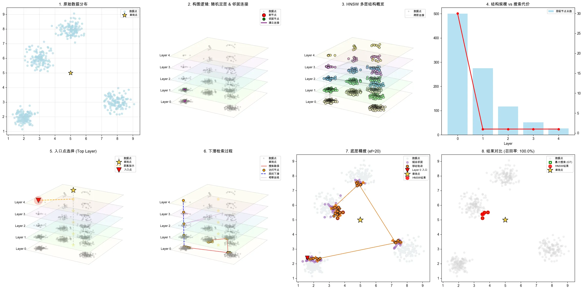
3.4参数影响分析
def analyze_hnsw_parameters(): """分析HNSW参数对性能的影响""" data = generate_sample_data(1000, 2) query = np.array([5.0, 5.0]) # 测试不同参数组合 parameter_combinations = [ {'M': 5, 'ef_construction': 30, 'ef_search': 20}, {'M': 10, 'ef_construction': 50, 'ef_search': 30}, {'M': 15, 'ef_construction': 100, 'ef_search': 50} ] results = [] for i, params in enumerate(parameter_combinations): print(f"\n测试参数组合 {i+1}: M={params['M']}, ef_construction={params['ef_construction']}") # 构建HNSW索引 hnsw = SimpleHNSW(max_elements=2000, M=params['M'], ef_construction=params['ef_construction'], max_layers=6) start_time = time.time() for point in data: hnsw.add_point(point) build_time = time.time() - start_time # 搜索 start_time = time.time() hnsw_results = hnsw.search(query, k=5, ef_search=params['ef_search']) search_time = time.time() - start_time # 计算召回率 distances = euclidean_distances([query], data)[0] bf_indices = np.argsort(distances)[:5] hnsw_indices_set = set(idx for idx, _ in hnsw_results) recall = len(hnsw_indices_set & set(bf_indices)) / 5 results.append({ 'params': params, 'build_time': build_time, 'search_time': search_time, 'recall': recall }) print(f"构建时间: {build_time:.4f}秒, 搜索时间: {search_time:.6f}秒, 召回率: {recall:.2%}") return results # 运行参数分析 param_results = analyze_hnsw_parameters()
输出结果
试参数组合 1: M=5, ef_construction=30 构建时间: 1.2516秒, 搜索时间: 0.000374秒, 召回率: 0.00% 测试参数组合 2: M=10, ef_construction=50 构建时间: 3.2875秒, 搜索时间: 0.000824秒, 召回率: 100.00% 测试参数组合 3: M=15, ef_construction=100 构建时间: 3.8578秒, 搜索时间: 0.001488秒, 召回率: 100.00%
核心参数的作用与结果分析
首先,理解两个核心参数的作用至关重要:
-
M(最大连接数):决定了图中每个节点可以和多少个邻居建立连接。M值越大,图的连通性越好,导航路径越多,但也会使索引更复杂、更占内存。
-
ef_construction(构建时候选集大小):控制着在插入一个新节点时,算法会在每一层探索多少个候选邻居来寻找最佳连接。此值越大,构建出的图质量通常越高,搜索精度越有保障,但索引的构建时间也会相应增加
现在我来尝试分析一下结果:
- 组合1 (
M=5, ef_construction=30):构建最快,但召回率崩溃- 这是典型的参数设置过于激进导致的问题。过小的
M和ef_construction使得构建出的图结构连通性极差。搜索时,算法可能迅速陷入局部最优解而无法找到真实的最近邻,从而导致召回率为0。虽然它的构建和搜索速度最快,但无法返回正确结果,这个组合在实际应用中是不可用的。
- 这是典型的参数设置过于激进导致的问题。过小的
- 组合2 (
M=10, ef_construction=50):性能的“甜蜜点”- 此组合在构建时间、搜索速度和召回率之间取得了极佳的平衡。它将
M和ef_construction提升到合理水平,成功构建出一个高质量的图结构,实现了100%的召回率。其搜索速度依然非常快,仅比组合1慢约0.00045秒,这个时间差对于大多数应用来说微不足道,却换来了结果准确性的质的飞跃。
- 此组合在构建时间、搜索速度和召回率之间取得了极佳的平衡。它将
- 组合3 (
M=15, ef_construction=100):精度优先,资源消耗增大- 进一步增大参数带来了边际效益递减。召回率维持在100%,但构建时间和搜索时间都有显著增加。这是因为算法需要处理更多的连接和候选点。这个组合适用于对召回率有极致要求且可以接受稍长延迟的场景