PowerUpSpeculativeDecodingInReinforcementLearning
文档摘要
Power Up Speculative Decoding In Reinforcement Learning TL;DR We introduce speculative decoding into the RL sampling process, achieving a significant improvement in sampling speed under appropriate batch sizes. Furthermore, the draft model is also updated during the training process.
Power Up Speculative Decoding In Reinforcement Learning
TL;DR
We introduce speculative decoding into the RL sampling process, achieving a significant improvement in sampling speed under appropriate batch sizes. Furthermore, the draft model is also updated during the training process. Compared to freezing the draft model, the accepted length is consistently maintained at a high level, generating long-term stable positive gains.
Speculative Decoding Documentation
Speculative Decoding in RL
Speculative Decoding is well-known as a clever inference acceleration technique. Specifically, during inference, instead of having the expensive target model decode token by token, a lightweight draft model first decodes and generates multiple tokens, which are then verified in batch by the large model. Tokens that pass verification are directly used as the final inference result, while failed tokens are resampled using the large model. Ideally, if all tokens generated by the draft model pass verification, the system can accept these k tokens at once, significantly improving inference efficiency. However, if the discrepancy between the draft model and the target model is too large, resulting in too few verified tokens, it might conversely have a negative effect.
Speculative Decoding, this double-edged sword, has already seen significant application in industrial-grade inference engines and also holds enticing potential in On-Policy RL. On one hand, speculative decoding can significantly accelerate the rollout sampling process, and the sampled tokens are, in distribution, identical to those from the target model. In addition, long-tail trajectories significantly reduce the effective parallelism during RL rollouts, making it difficult to fully saturate hardware compute; this regime naturally matches the application scenario of speculative decoding. Of course, all this is premised on the sampling probability difference between the draft model and the target model being within a reasonable range—if the policy difference between the two is too large, the acceptance rate of tokens predicted by the draft model will plummet.
This is the problem solved in this article—we introduce speculative decoding into the RL sampling process and synchronously update the draft model as training progresses, stably improving sampling speed.
This feature has already been merged into miles main branch and is available out of the box. See the same documentation for usage details.
Online SFT for Draft Model
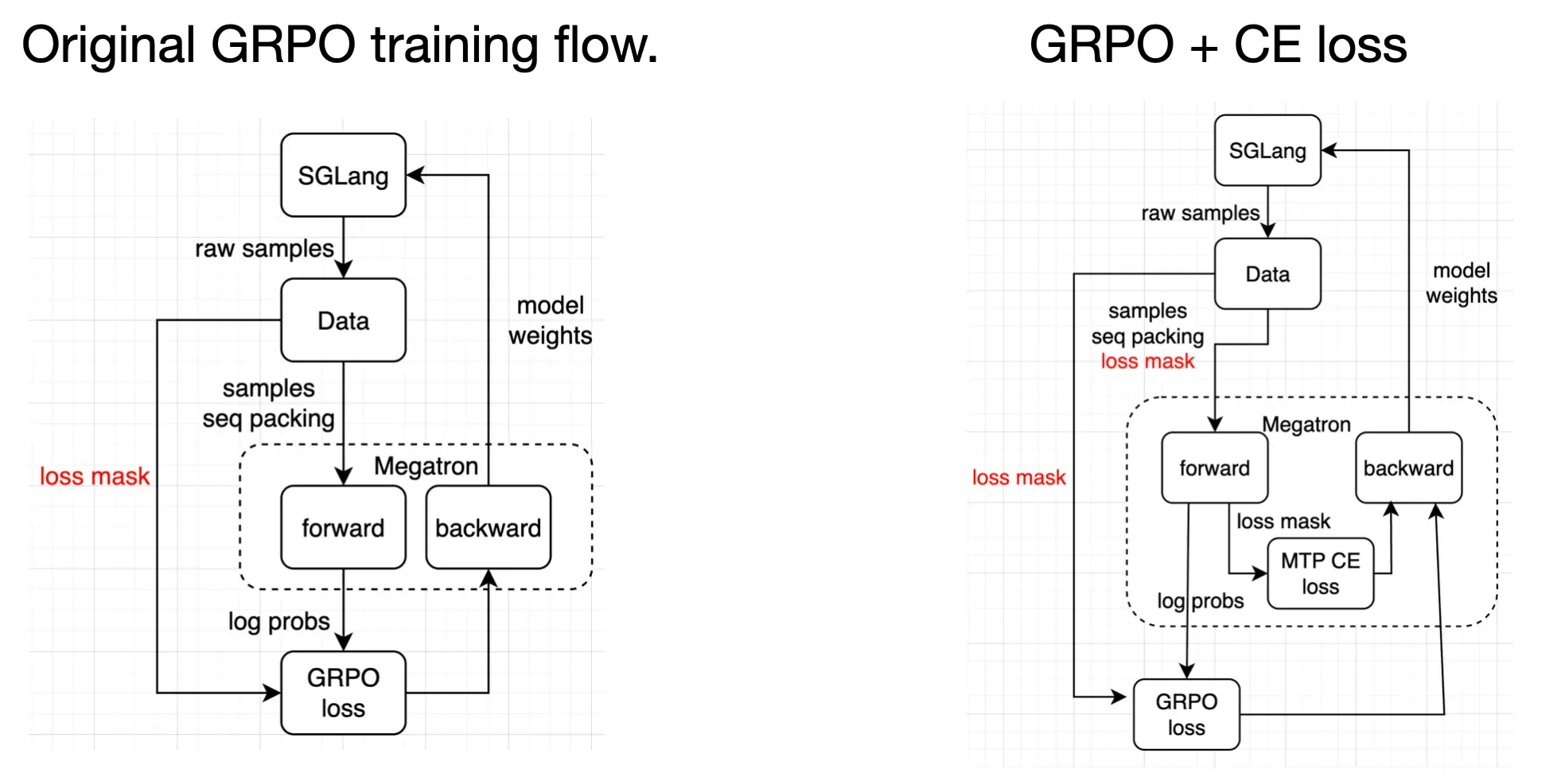
Megatron added support for EAGLE MTP SFT in v0.12.0rc3. Based on this, we consider performing online SFT on the draft model during the training process. Specifically, we add a new cross entropy loss (CE Loss) flow inside the Megatron backend, using the target model's hidden state and generated tokens as input to the MTP layer (i.e., the draft model), with the expectation that the MTP layer can accurately predict the next token that the target model will actually generate. When the target model's GPRO Loss calculation is complete and backward() is called, it triggers the backpropagation of both the target model's GPRO Loss and the MTP CE Loss simultaneously. The specific process is as follows:
Constructing the Training Objective
To analyze our loss construction, let's first describe the training objective for the draft model. In a standard autoregressive model, our training objective is to use the input at time t to predict the token at time t+1, i.e., input(t) -> output(t+1). In contrast, mainstream speculative decoding uses EAGLE MTP as the draft model, and its prediction target is the token at time t+2, i.e., Input(t) + Input(t+1) → Output(t+2).
Specifically, assume the target model outputs tokens a, b, c. Correspondingly, we have hidden states at three token positions, denoted as h(a), h(b), h(c), and token embedding information at three positions, denoted as e(a), e(b), e(c). The MTP layer's objective is to predict the token at time c given the target model's "thought" (hidden state) at time a and the input (embedding) at time b.
Constructing the Training Input
Based on the analysis above, the MTP layer receives two inputs:
- Target model's hidden state: Obtained directly from the target model's forward process.
- Token embedding: Shift the tokens obtained from the target model to the left once (
roll_tensor) and then pass them through the embedding layer.
Assume the target model's generated sequence is [a, b, c, d, e]:
target_model_hidden_state = [h(a), h(b), h(c), h(d), h(e)] rolled_tokens = roll_tensor([a, b, c, d, e], shift=-1) = [b, c, d, e, ❌] token_embedding = e(rolled_tokens) = [e(b), e(c), e(d), e(e), ❌]
Next, the MTP inputs token_embedding and target_model_hidden_state and outputs draft_hidden_state. The draft_hidden_state is passed through the lm head (shared with the target model) to get the log probs for each token. At this point, we expect the MTP's output to be [c, d, e, ❌, ❌], which is the result of shifting rolled_tokens to the left once more. This is used as the labels to calculate the CE loss.
Constructing the Training Flow
draft_hidden_state = mtp(concat([token_embedding, target_model_hidden_state])) mtp_logits = shared_output_layer(draft_hidden_state) labels = roll_tensor(rolled_tokens, shift=-1) = [c, d, e, ❌, ❌] mtp_loss = cross_entropy(labels, mtp_logits)
As mentioned earlier, we add a new SFT CE Loss flow in Megatron. After Megatron returns the target model's log probs, the GRPO Loss is calculated, and then backward() is called, triggering the backward pass for both the GRPO Loss and the CE Loss.
To prevent conflicts between the two losses, we detach the hidden state passed from the main model to the MTP, as well as the lm head and embedding shared by the main model and the MTP.
Implementation Results
We conducted tests on an H200 cluster based on the Mimo-7B-RL model, using the DAPO-Math-17k dataset, with max response length = 24k.
- Experimental group – Online SFT spec: Enable the MTP layer for speculative decoding and train the MTP layer.
- Baseline 1 – Frozen spec: Enable the MTP layer for speculative decoding, but do not train the MTP layer.
- Baseline 2 – No spec: Speculative decoding disabled.
The results are as follows:
| Experimental Group – Online SFT spec | Baseline 1 – Frozen spec | Baseline 2 – No spec | |
|---|---|---|---|
| Rollout Throughput (tokens/s) | 1667 | 1464 | 1219 |
| Long-tail Efficiency (tokens/s) | 65 | 57 | 47 |
| Training Time (s) | 148 | 143 | 141 |
- MTP learns steadily
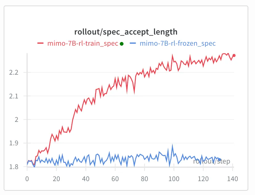
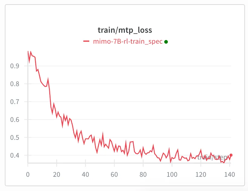
After enabling MTP training, the accept length steadily increases, and the MTP loss decreases.
- Rollout performance
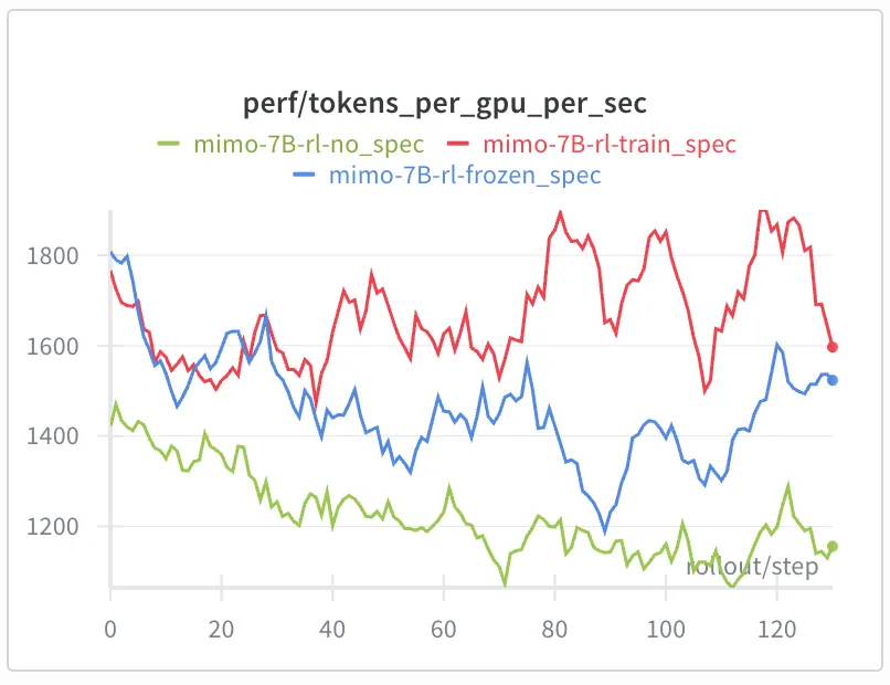
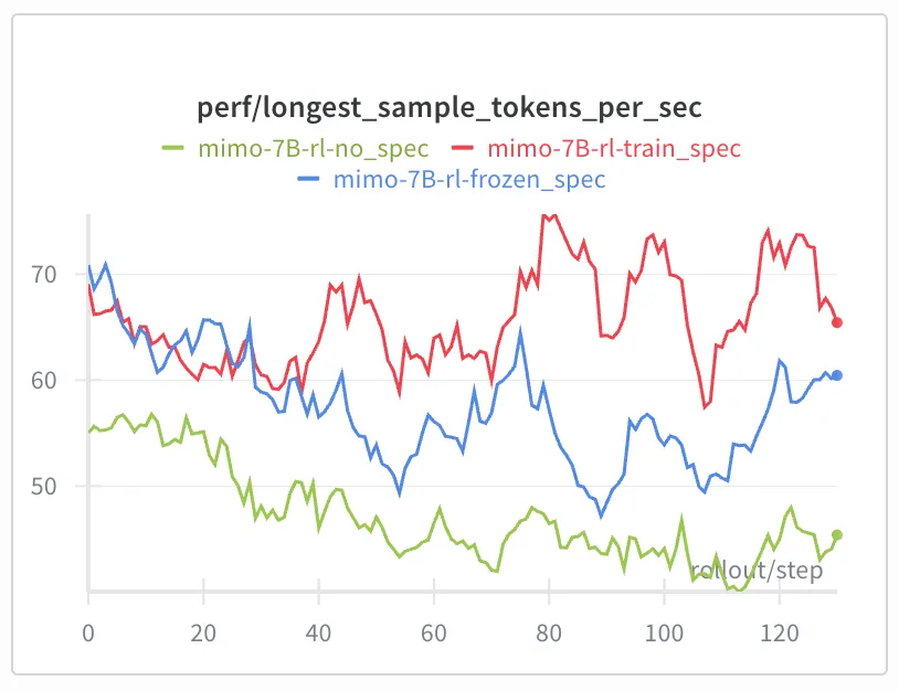
Compared to disabling speculative decoding, training spec provides about 35% improvement in rollout throughput overall. Compared to frozen spec, training spec yields about 14% improvement on average. This gap becomes more pronounced in the later stages of training, where training spec outperforms frozen spec by up to 25%.
- Training time
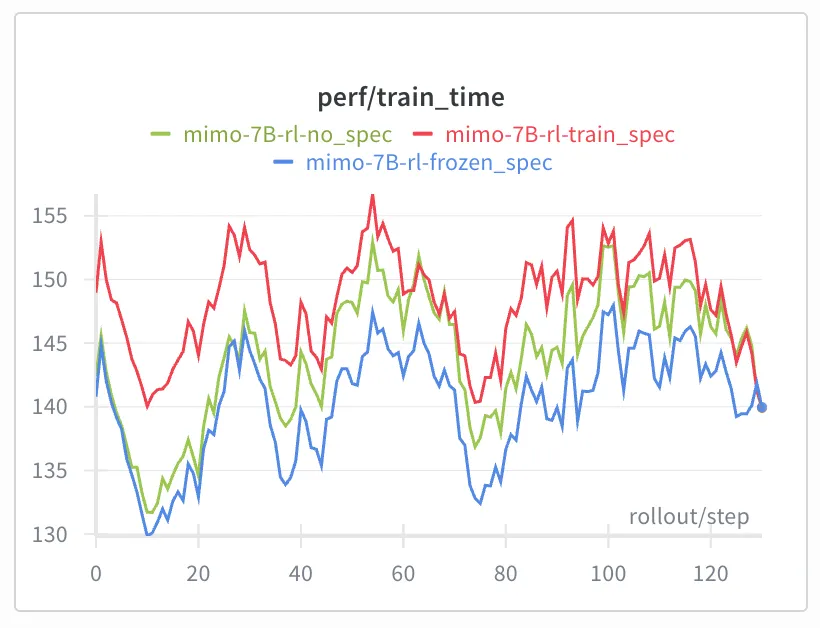
Because we additionally train the MTP layer, training time increases slightly. However, the time saved on faster rollouts more than offsets this overhead, leading to a clear net speedup.
- Training effectiveness
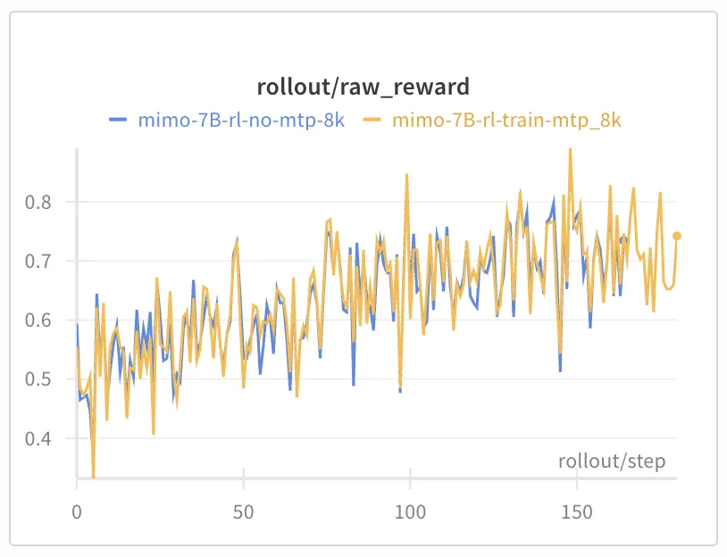
As theoretically expected, introducing speculative decoding into the sampling process does not affect the main model's sampling or training quality. The reward curves remain consistent across settings:
Appendix: Engineering Practices
Sequence Packing
In a naive training pipeline, the input sequence has dimensions [bs, seq]. Since different sequences have varying lengths, they must be padded to the longest sequence in the seq dimension, which causes each sample to waste a certain amount of memory. To achieve optimal training throughput, we flatten a batch to bs = 1. Specifically, we use sequence packing in the seq dimension to concatenate sequences before inputting them into Megatron.
Although Megatron supports MTP SFT, it does not yet support MTP training in sequence packing scenarios. To support Megatron's MTP, we implemented the roll_tensor function for MTP, which shifts the input sequence one position to the left and sets the end to 0. Handling context parallelism is crucial here.
Without sequence packing, Megatron's implementation of roll_tensor is as follows:
- When CP = 1, it calls the naive
roll_tensor, usingtorch.rollto shift the entire sequence one position to the left and setting the end to 0. - When CP > 1:
- First, a naive
roll_tensoris performed inside each CP chunk. (In the diagram below: Input → Roll each tensor individually) - The left chunk of each rank sends its tail element to the left chunk of the previous rank. (In the diagram below, bottom part of Handle boundaries: 12 → 8 → 4 → 0)
- The right chunk of each rank sends its tail element to the right chunk of the next rank. (In the diagram below, bottom part of Handle boundaries: 28 → 24 → 20 → 16)
rank = 0andrank = n-1need to be handled separately as boundaries.
- First, a naive

In miles, CP splitting is performed before sequence packing:
- First, each sequence is padded, split according to CP rules, and concatenated across ranks (to get aligned CP blocks on each rank).
- Then, within each rank, sequence packing is applied to multiple sequences, concatenating them into a continuous tensor.
Therefore, in the sequence packing scenario, the original roll_tensor logic can be almost directly reused: just execute roll_tensor for each sequence separately.
Loss mask processing
The loss mask involves two issues:
- How the loss mask is passed to Megatron
We just mentioned that MTP training adds a new MTP CE Loss Flow, and the CE loss is calculated within Megatron. Originally (without MTP), miles only needed to call Megatron to compute logits, so it didn't need to consider the loss mask within Megatron. But now, the MTP CE Loss must be calculated in Megatron—which requires a loss mask.
Therefore, we need to process the original loss mask: pad the prompt part, split it according to CP rules, pad the end to align with input ids, and then pass it to Megatron. The slice_with_cp() API in miles can be directly reused for CP splitting.
- The intersection problem of the loss mask
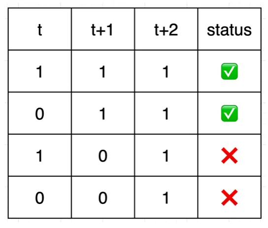
First, the CE loss mask must align with the shifted labels, so it needs to be shifted twice. If the input loss mask is [1, 0, 1, 1, 0], after two shifts, it should be [1, 1, 0, ❌, ❌].
However, in training, we already assume that [b, c, d, e, ❌] is generated from [a, b, c, d, e], and then we predict [c, d, e, ❌, ❌] based on [Ha, Hb, Hc, Hd, He] and [Eb, Ec, Ed, Ee, ❌], as shown in the figure. But if the mask for b is 0, then b is definitely not a token the model needs to generate, b could not have been generated from a, and it's even more impossible for the MTP to generate c based on Ha and Eb.
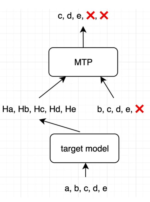
Therefore, to perform MTP at position t, we need the "intermediate token" at t+1 to be valid, and we also need the "target token" at t+2 to be valid, but we don't need to care if t is valid (because t is not involved in the calculation); So, we take the intersection of the two shifted masks. We need to combine the once-shifted loss mask `[0, 1, 1, 0, ❌]` and the twice-shifted mask `[1, 1, 0, ❌, ❌]` to get `[0, 1, 0, ❌, ❌]`.
loss_mask_1 = roll_tensor(loss_mask, shift=-1) loss_mask_2 = roll_tensor(loss_mask_1, shift=-1) mtp_loss_mask = loss_mask_2 * loss_mask_1
The final state is as follows:
Truncating lm_head and embedding
In MTP training, we want to reuse the main model's LM head and embedding, but we do not want the auxiliary MTP loss to update these parameters—they should only be driven by the main LM loss. At the same time, the hidden states produced by the MTP branch still need to receive gradients; otherwise, the MTP layers themselves would not learn anything.
To achieve this, we explicitly cut the gradient paths from the MTP branch to the main model's parameters, while keeping gradients flowing within the MTP layers. In practice, we do three things:
-
Cut gradients to the main model and embedding
decoder_input = embedding(input_ids=input_ids, position_ids=position_ids) decoder_input = decoder_input.detach() hidden_states = make_viewless_tensor( inp=hidden_states, requires_grad=True, keep_graph=False, )Here we first perform a normal embedding lookup, then immediately call
detach()ondecoder_input. The forward values remain unchanged—we still use the main model's embedding weights. However, when backpropagating from the MTP loss, gradients will no longer flow back into the embedding weights; on the MTP branch, the embedding is effectively a read-only constant.hidden_statesis handled similarly: we re-wrap it viamake_viewless_tensorso that it can receive gradients on this branch without treating it as a view of the original tensor. -
Cut gradients to the LM head
for mtp_layer_number in range(self.config.mtp_num_layers): # 1. Get all parameters of output_layer and detach them output_layer_params = { k: v.detach() for k, v in self.output_layer.named_parameters() } # 2. Get all buffers (e.g., LayerNorm running stats) output_layer_buffers = dict(self.output_layer.named_buffers()) # 3. Use functional_call to invoke output_layer as a "pure function" mtp_logits, _ = torch.func.functional_call( self.output_layer, {**output_layer_params, **output_layer_buffers}, (hidden_states_list[mtp_layer_number + 1],), { # tied embedding should also be detached to avoid being updated by MTP loss "weight": output_weight.detach() if output_weight else None, "runtime_gather_output": runtime_gather_output, }, )The key points here are:
-
We detach at the parameter level, not at the output level. Both
output_layer_paramsandoutput_weightare detached once. The computation graph is cut at the LM head's parameters, so the gradient from the MTP loss with respect toself.output_layer's parameters is effectively 0. -
We use
torch.func.functional_callfor a “functional” invocation:functional_call(module, params_and_buffers, args, kwargs)can be viewed conceptually as calling a pure function
f(params, buffers, inputs), where this invocation uses an explicitly provided parameter dictionary instead of the parameters stored inside the module.This has two benefits:
- We do not modify the parameters stored on
self.output_layernor theirrequires_gradflags. The main LM loss can still update the same LM head as usual. - On the MTP branch, we temporarily “swap in” a detached view of the parameters for this forward pass only, so gradients from the MTP loss do not flow into the LM head parameters.
- We do not modify the parameters stored on
-
We also detach the tied embedding weight (
output_weight) to ensure it is not updated by the MTP loss.
-
Mimo-7B-RL Model Support
Megatron's default MTP input concatenation is [target_token_embed, hidden_state], which works for DeepSeek and GLM. However, when testing the feature, due to limited computing resources and for rapid validation, we used the Mimo-7B-RL small model (possibly the only small model with MTP). Unfortunately, we found that when training Mimo directly with Megatron, the loss was particularly high.
We finally discovered that Mimo's MTP input format is [hidden_state, target_token_embed], the complete opposite of DeepSeek and GLM. After finding the cause, the solution was very direct: swap the parameter values of the first and second halves of eh_proj before Megatron checkpoint conversion and before Megatron updates weights to SGLang.
Acknowledgements
Thanks to @Zilin Zhu @Shenggui Li @Tom for their technical guidance
Thanks to @Chenyang Zhao @Mao Cheng for the complete rewrite of this blog
Thanks to @Yuzhen Zhou @Mao Cheng @Ruiguo Yang @Ji Li @Qiaolin Yu @Kangrui Du @Jin Pan @Xinyuan Tong for their collaborative development.