第25章 循环神经网络
文档摘要
第25章循环神经网络 习题25.1   Jordan提出的循环神经网络如图25.15所示。试写出这种神经网络的公式,并与Elman提出的简单循环神经网络做比较。 25-1.png 解答: 解答思路: 给出简单循环神经网络(S-RNN)的定义 给出Jordan提出的循环神经网络的公式 比较Jordan RNN和S-RNN 解答步骤: 第1步:简单循环神经网络(S-RNN)的定义   根据书中第25.1.1节的定义25.1的简单循环神经网络(即Elman提出的简单循环神经网络)的定义: 定义25.1(简单循环神经网络) 称以下的神经网络为简单循环神经网络。神经网络以序列数据$x1, x2, \cdots, xT$为输入,每一项是一个实数向量。
第25章循环神经网络
习题25.1
Jordan提出的循环神经网络如图25.15所示。试写出这种神经网络的公式,并与Elman提出的简单循环神经网络做比较。
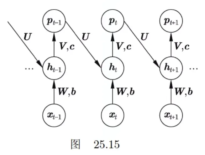
解答:
解答思路:
- 给出简单循环神经网络(S-RNN)的定义
- 给出Jordan提出的循环神经网络的公式
- 比较Jordan RNN和S-RNN
解答步骤:
第1步:简单循环神经网络(S-RNN)的定义
根据书中第25.1.1节的定义25.1的简单循环神经网络(即Elman提出的简单循环神经网络)的定义:
定义25.1(简单循环神经网络) 称以下的神经网络为简单循环神经网络。神经网络以序列数据x_1, x_2, \cdots, x_T为输入,每一项是一个实数向量。在每一个位置上重复使用同一个神经网络结构。在第t个位置上(t = 1, 2, \cdots, T),神经网络的隐层或中间层以x_t和h_{t-1}为输入,以h_t为输出,其间有以下关系成立:
h_t = \tanh (U \cdot h_{t - 1} + W \cdot x_t + b) \tag{25.1}
p_t = \text{softmax} (V \cdot h_t + c) \tag{25.2}
r_t = U \cdot h_{t - 1} + W \cdot x_t + b \tag{25.3}
h_t = \tanh(r_t) \tag{25.4}
z_t = V \cdot h_t + c \tag{25.5}
p_t = \text{softmax}(z_t) \tag{25.6}
\boldsymbol{r}t = \boldsymbol{U} \cdot \boldsymbol{p}{t-1} + W \cdot \boldsymbol{x}_t + \boldsymbol{b} \
\boldsymbol{h}_t = \tanh (\boldsymbol{r}_t) \
\boldsymbol{z}_t = V \cdot \boldsymbol{h}_t + \boldsymbol{c} \
\boldsymbol{p}t = \text{softmax} (\boldsymbol{z}{t})
\mu = \frac{1}{m} \sum_{j = 1}^m z_j \tag{23.65}
\sigma^2 = \frac{1}{m - 1} \sum_{j = 1}^m (z_j - \mu)^2 \tag{23.66}
\bar{z}_j = \frac{z_j - \mu}{\sqrt{\sigma^2 + \epsilon}}, \ j= 1, 2, \cdots, m \tag{23.67}
\tilde{z}_j = \gamma \cdot \bar{z}_j + \beta, \ j = 1, 2, \cdots, m \tag{23.68}
\tilde{z}^{(l)} = \gamma \cdot \frac{z^{(l)}-\mu^{(l)}}{\sqrt{\sigma^{(l)}+\epsilon}} + \beta
z_t=U h_{t-1}+W x_t + b\
h_t=f\left(L N_{\gamma, \beta}\left(z_t\right)\right)
\boldsymbol{h}^{(0)} = \boldsymbol{x}
z^{(t)} = \boldsymbol{W}^{(t)} \boldsymbol{h}^{(t - 1)} + \boldsymbol{b}^{(t)} \
\boldsymbol{h}^{(t)} = a (z^{(t)})
f(\boldsymbol{x}) = \boldsymbol{h}^{(s)}
\boldsymbol{\delta}^{(s)} = \boldsymbol{h}^{(s)} - \boldsymbol{y}
\nabla_{\boldsymbol{W}^{(t)}} L = \boldsymbol{\delta}^{(t)} \cdot {\boldsymbol{h}^{(t - 1)}}^T \
\nabla_{\boldsymbol{b}^{(t)}} L = \boldsymbol{\delta}^{(t)}
\boldsymbol{W}^{(t)} \leftarrow \boldsymbol{W}^{(t)} - \eta \nabla_{\boldsymbol{W}^{(t)}} L \
\boldsymbol{b}^{(t)} \leftarrow \boldsymbol{b}^{(t)} - \eta \nabla_{\boldsymbol{b}^{(t)}} L
\boldsymbol{\delta}^{(t - 1)} = \frac{\partial a}{\partial z^{(t - 1)}} \odot \left ( {\boldsymbol{W}^{(t)}}^T \cdot \boldsymbol{\delta}^{(t)} \right )
r_t = U \cdot h_{t - 1} + W \cdot x_t + b \
h_t = \tanh (r_t) \
z_t = V \cdot h_t + c \
p_t = \text{softmax}(z_t)
\frac{\partial{L}}{\partial{z_t}} = y_t - p_t
\frac{\partial{L}}{\partial{r_t}} = \text{diag}(\boldsymbol{1} - \tanh^2 r_t) \cdot U^T \cdot \frac{\partial{L}}{\partial{r_{t+1}}} + \text{diag}(\boldsymbol{1} - \tanh^2 r_t) \cdot V^T \cdot \frac{\partial{L}}{\partial{z_t}}
\frac{\partial{L}}{\partial{r_T}} = \text{diag}(\boldsymbol{1} - \tanh^2 r_T) \cdot V^T \cdot \frac{\partial{L}}{\partial{z_T}}
\frac{\partial{L}}{\partial{c}} = \sum_{t = 1}^T \frac{\partial{L}}{\partial{z_t}} \
\frac{\partial{L}}{\partial{V}} = \sum_{t = 1}^T \frac{\partial{L}}{\partial{z_t}} \cdot h_t^T \
\frac{\partial{L}}{\partial{b}} = \sum_{t = 1}^T \frac{\partial{L}}{\partial{r_t}} \
\frac{\partial{L}}{\partial{U}} = \sum_{t = 1}^T \frac{\partial{L}}{\partial{r_t}} \cdot h_{t - 1}^T \
\frac{\partial{L}}{\partial{W}} = \sum_{t = 1}^T \frac{\partial{L}}{\partial{r_t}} \cdot x_t^T
c \leftarrow c - \eta \frac{\partial{L}}{\partial{c}} \
V \leftarrow V - \eta \frac{\partial{L}}{\partial{V}} \
b \leftarrow b - \eta \frac{\partial{L}}{\partial{b}} \
W \leftarrow W - \eta \frac{\partial{L}}{\partial{W}} \
U \leftarrow U - \eta \frac{\partial{L}}{\partial{U}}
i_t = \sigma(U_i \cdot h_{t - 1} + W_i \cdot x_t + b_i) \tag{25.20}
f_t = \sigma(U_f \cdot h_{t - 1} + W_f \cdot x_t + b_f) \tag{25.21}
o_t = \sigma(U_o \cdot h_{t - 1} + W_o \cdot x_t + b_o) \tag{25.22}
\tilde{c}t = \tanh (U_c \cdot h{t - 1} + W_c \cdot x_t + b_c) \tag{25.23}
c_t = i_t \odot \tilde{c}t + f_t \odot c{t - 1} \tag{25.24}
h_t = o_t \odot \tanh(c_t) \tag{25.25}
i_t = \sigma\left(\tilde{i}t\right) = \sigma(U_i \cdot h{t - 1} + W_i \cdot x_t + b_i) \
f_t = \sigma\left(\tilde{f}t\right) = \sigma(U_f \cdot h{t - 1} + W_f \cdot x_t + b_f) \
o_t = \sigma\left(\tilde{o}t\right) = \sigma(U_o \cdot h{t - 1} + W_o \cdot x_t + b_o) \
g_t = \tanh(\tilde{g}t) = \tilde{c}t = \tanh (U_c \cdot h{t - 1} + W_c \cdot x_t + b_c) \
c_t = i_t \odot g_t + f_t \odot c{t - 1} \
h_t = o_t \odot \tanh(c_t) \
z_t = V \cdot h_t + c \
p_t = \text{softmax}(z_t)
\frac{\partial L}{\partial h_{t}}
= \frac{\partial L}{\partial z_t} V^T + \frac{\partial L}{\partial \tilde{o}{t+1}} U_o^T + \frac{\partial L}{\partial \tilde{f}{t+1}} U_f^T + \frac{\partial L}{\partial \tilde{i}{t+1}} U_i^T + \frac{\partial L}{\partial \tilde{g}{t+1}} U_c^T
\begin{aligned}
\frac{\partial L}{\partial c_t}
&= \frac{\partial L}{\partial \tanh (c_t)} \frac{d \tanh(c_t)}{d c_t} + \frac{\partial L}{\partial c_{t+1}} \odot f_{t+1} \
&= \left( \frac{\partial L}{\partial h_t} \odot o_t \right ) \cdot \text{diag}(\boldsymbol{1} - \tanh^2 c_t) + \frac{\partial L}{\partial c_{t + 1}} \odot f_{t + 1}
\end{aligned}
\begin{aligned}
\frac{\partial L}{\partial \tilde{g}_t}
&= \frac{\partial L}{\partial g_t} ( 1 - g_t^2 ) \
&= (1 - g_t^2) \cdot \frac{\partial L}{\partial c_t} \odot i_t
\end{aligned}
\begin{aligned}
\frac{\partial L}{\partial \tilde{i}_t}
&= \frac{\partial L}{\partial i_t} i_t ( 1 - i_t ) \
&= i_t ( 1 - i_t ) \cdot \frac{\partial L}{\partial c_t} \odot g_t
\end{aligned}
\begin{aligned}
\frac{\partial L}{\partial \tilde{f}t}
&= \frac{\partial L}{\partial f_t} f_t (1 - f_t) \
&= f_t (1 - f_t) \cdot \frac{\partial L}{\partial c_t} \odot c{t-1}
\end{aligned}
\begin{aligned}
\frac{\partial L}{\partial \tilde{o}_t}
&= \frac{\partial L}{\partial o_t} i_t (1 - o_t) \
&= i_t (1 - o_t) \cdot \frac{\partial L}{\partial h_t} \odot \tanh (c_t)
\end{aligned}
\frac{\partial L}{\partial x_t} = \frac{\partial L}{\partial \tilde{o}_t} W_o^T + \frac{\partial L}{\partial \tilde{f}_t} W_f^T + \frac{\partial L}{\partial \tilde{i}_t} W_i^T + \frac{\partial L}{\partial \tilde{g}_t} W_c^T
\frac{\partial L}{\partial U_o} = \sum_{t=1}^T \frac{\partial L}{\partial \tilde{o}{t + 1}} \cdot h_t^T \
\frac{\partial L}{\partial U_f} = \sum{t=1}^T \frac{\partial L}{\partial \tilde{f}_{t + 1}} \cdot h_t^T \
\frac{\partial L}{\partial U_i} = \sum_{t=1}^T \frac{\partial L}{\partial \tilde {i}_{t + 1}} \cdot h_t^T \
\frac{\partial L}{\partial U_c} = \sum_{t=1}^T \frac{\partial L}{\partial \tilde{g}_{t + 1}} \cdot h_t^T
\frac{\partial L}{\partial V} = \sum_{t=1}^T \frac{\partial L}{\partial z_t} \cdot h_t^T
\frac{\partial L}{\partial W_o} = \sum_{t=1}^T \frac{\partial L}{\partial \tilde{o}t} \cdot x_t^T \
\frac{\partial L}{\partial W_f} = \sum{t=1}^T \frac{\partial L}{\partial \tilde{f}_t} \cdot x_t^T \
\frac{\partial L}{\partial W_i} = \sum_{t=1}^T \frac{\partial L}{\partial \tilde{i}_t} \cdot x_t^T \
\frac{\partial L}{\partial W_c} = \sum_{t=1}^T \frac{\partial L}{\partial \tilde{g}_t} \cdot x_t^T
\frac{\partial L}{\partial b_i} = \sum_{t=1}^T \frac{\partial L}{\partial \tilde{i}t} \
\frac{\partial L}{\partial b_f} = \sum{t=1}^T \frac{\partial L}{\partial \tilde{f}_t} \
\frac{\partial L}{\partial b_o} = \sum_{t=1}^T \frac{\partial L}{\partial \tilde{o}_t} \
\frac{\partial L}{\partial b_c} = \sum_{t=1}^T \frac{\partial L}{\partial \tilde{g}_t}
i_t = \sigma\left(\tilde{i}t\right) = \sigma(U_i \cdot h{t - 1} + W_i \cdot x_t + b_i) \
f_t = \sigma\left(\tilde{f}t\right) = \sigma(U_f \cdot h{t - 1} + W_f \cdot x_t + b_f) \
o_t = \sigma\left(\tilde{o}t\right) = \sigma(U_o \cdot h{t - 1} + W_o \cdot x_t + b_o) \
g_t = \tanh(\tilde{g}t) = \tilde{c}t = \tanh (U_c \cdot h{t - 1} + W_c \cdot x_t + b_c) \
c_t = i_t \odot g_t + f_t \odot c{t - 1} \
h_t = o_t \odot \tanh(c_t) \
z_t = V \cdot h_t + c \
p_t = \text{softmax}(z_t)
\frac{\partial{L}}{\partial{z_t}} = y_t - p_t
\frac{\partial L}{\partial \tilde{i}_t} = i_t ( 1 - i_t ) \cdot \frac{\partial L}{\partial c_t} \odot g_t \
\frac{\partial L}{\partial \tilde{f}t} = f_t (1 - f_t) \cdot \frac{\partial L}{\partial c_t} \odot c{t-1} \
\frac{\partial L}{\partial \tilde{o}_t} = i_t (1 - o_t) \cdot \frac{\partial L}{\partial h_t} \odot \tanh (c_t)
\frac{\partial L}{\partial c_t} = \left( \frac{\partial L}{\partial h_t} \odot o_t \right ) \cdot \text{diag}(\boldsymbol{1} - \tanh^2 c_t) + \frac{\partial L}{\partial c_{t + 1}} \odot f_{t + 1} \
\frac{\partial L}{\partial h_{t}}
= \frac{\partial L}{\partial z_t} V^T + \frac{\partial L}{\partial \tilde{o}{t+1}} U_o^T + \frac{\partial L}{\partial \tilde{f}{t+1}} U_f^T + \frac{\partial L}{\partial \tilde{i}{t+1}} U_i^T + \frac{\partial L}{\partial \tilde{g}{t+1}} U_c^T \
g_t = \tanh (U_c \cdot h_{t - 1} + W_c \cdot x_t + b_c)
\frac{\partial L}{\partial \tilde{i}_T} = i_T (1 - i_T) \cdot \frac{\partial L}{\partial c_T} \odot g_T \
\frac{\partial L}{\partial \tilde{f}T} = f_T (1 - f_T) \cdot \frac{\partial L}{\partial c_T} \odot c{T-1} \
\frac{\partial L}{\partial \tilde{o}_T} = i_T (1 - o_T) \cdot \frac{\partial L}{\partial h_T} \odot \tanh (c_T)
\frac{\partial L}{\partial c_T} = \left ( \frac{\partial L}{\partial h_T} \odot o_T \right) \cdot \text{diag} (\boldsymbol{1} - \tanh^2 c_T) \
\frac{\partial L}{\partial h_T} = \frac{\partial L}{\partial z_T} V^T \
g_T = \tanh (U_c \cdot h_{T - 1} + W_c \cdot x_T + b_c)
\frac{\partial L}{\partial U_o} = \sum_{t=1}^T \frac{\partial L}{\partial \tilde{o}{t + 1}} \cdot h_t^T \
\frac{\partial L}{\partial U_f} = \sum{t=1}^T \frac{\partial L}{\partial \tilde{f}_{t + 1}} \cdot h_t^T \
\frac{\partial L}{\partial U_i} = \sum_{t=1}^T \frac{\partial L}{\partial \tilde {i}_{t + 1}} \cdot h_t^T \
\frac{\partial L}{\partial U_c} = \sum_{t=1}^T \frac{\partial L}{\partial \tilde{g}_{t + 1}} \cdot h_t^T
\frac{\partial L}{\partial V} = \sum_{t=1}^T \frac{\partial L}{\partial z_t} \cdot h_t^T
\frac{\partial L}{\partial W_o} = \sum_{t=1}^T \frac{\partial L}{\partial \tilde{o}t} \cdot x_t^T \
\frac{\partial L}{\partial W_f} = \sum{t=1}^T \frac{\partial L}{\partial \tilde{f}_t} \cdot x_t^T \
\frac{\partial L}{\partial W_i} = \sum_{t=1}^T \frac{\partial L}{\partial \tilde{i}_t} \cdot x_t^T \
\frac{\partial L}{\partial W_c} = \sum_{t=1}^T \frac{\partial L}{\partial \tilde{g}_t} \cdot x_t^T
\frac{\partial L}{\partial b_i} = \sum_{t=1}^T \frac{\partial L}{\partial \tilde{i}t} \
\frac{\partial L}{\partial b_f} = \sum{t=1}^T \frac{\partial L}{\partial \tilde{f}_t} \
\frac{\partial L}{\partial b_o} = \sum_{t=1}^T \frac{\partial L}{\partial \tilde{o}_t} \
\frac{\partial L}{\partial b_c} = \sum_{t=1}^T \frac{\partial L}{\partial \tilde{g}_t}
U_o \leftarrow U_o - \eta \frac{\partial L}{\partial U_o} \
U_f \leftarrow U_f - \eta \frac{\partial L}{\partial U_f} \
U_i \leftarrow U_i - \eta \frac{\partial L}{\partial U_i} \
U_c \leftarrow U_c - \eta \frac{\partial L}{\partial U_c}
V \leftarrow V - \eta \frac{\partial L}{\partial V}
W_o \leftarrow W_o - \eta \frac{\partial L}{\partial W_o} \
W_f \leftarrow W_f - \eta \frac{\partial L}{\partial W_f} \
W_i \leftarrow W_i - \eta \frac{\partial L}{\partial W_i} \
W_c \leftarrow W_c - \eta \frac{\partial L}{\partial W_c}
b_o \leftarrow b_o - \eta \frac{\partial L}{\partial b_o} \
b_f \leftarrow b_f - \eta \frac{\partial L}{\partial b_f} \
b_i \leftarrow b_i - \eta \frac{\partial L}{\partial b_i} \
b_c \leftarrow b_c - \eta \frac{\partial L}{\partial b_c}
c_t = i_t \odot \tilde{c}t + f_t \odot c{t - 1} = \sum_{i = 1}^t \left( \prod_{j = i + 1}^t f_j \odot i_i \right) \odot \tilde{c}i = \sum{i = 1}^t w_i^t \odot \tilde{c}_i \tag{25.26}
c_t = i_t \odot \tilde{c}t + f_t \odot c{t - 1} \tag{1}
c_{t-1} = i_{t-1}\odot\tilde{c}{t-1} + f{t-1} \odot c_{t-2} \tag{2}
\begin{aligned}
c_t
&= i_t \odot \tilde{c}t + f_t \odot (i{t-1} \odot \tilde{c}{t-1} + f{t-1}\odot c_{t-2}) \
&= i_t \odot \tilde{c}t + f_t \odot i{t-1} \odot \tilde{c}{t-1} + f_t \odot f{t-1} \odot c_{t-2}
\end{aligned} \tag{3}
\begin{aligned}
c_t
&= i_t \odot \tilde{c}t + f_t \odot i{t-1} \odot \tilde{c}{t-1} + f_t \odot f{t-1} \odot c_{t-2} \
&= i_t \odot \tilde{c}t + f_t \odot i{t-1} \odot \tilde{c}{t-1} + f_t \odot f{t-1} \odot (i_{t-2} \odot \tilde{c}{t-2} + f{t-2} \odot c_{t-3}) \
&= i_t \odot \tilde{c}t + f_t \odot i{t-1} \odot \tilde{c}{t-1} + f_t \odot f{t-1} \odot i_{t-2} \odot \tilde{c}{t-2} + f_t \odot f{t-1} \odot f_{t-2} \odot c_{t-3} \
&= i_t \odot \tilde{c}t + f_t \odot i{t-1} \odot \tilde{c}{t-1} + f_t \odot f{t-1} \odot i_{t-2} \odot \tilde{c}{t-2} + \cdots + f_t \odot f{t-1} \odot f_3 \odot i_2 \odot \tilde{c}2 + f_t \odot f{t-1} \odot f_2 \odot c_1 \
&= \sum_{i=2}^{t}(\prod_{j=i+1}^{t} f_j \odot i_i)\odot \tilde{c}_i + f_t \odot f_{t-1} \odot f_2 \odot c_1
\end{aligned}
\begin{aligned}
c_t
&= \sum_{i=2}^{t}(\prod_{j=i+1}^{t} f_j \odot i_i)\odot \tilde{c}_i + f_t \odot f_{t-1} \odot f_2 \odot c_1 \
&= \sum_{i=2}^{t}(\prod_{j=i+1}^{t} f_j \odot i_i)\odot \tilde{c}_i + f_t \odot f_{t-1} \odot f_2 \odot i_1 \odot \tilde{c}_1 \
&= \sum_{i=1}^{t}(\prod_{j=i+1}^{t} f_j \odot i_i)\odot \tilde{c}_i
\end{aligned}
w_i^t = \prod_{j=i+1}^{t} f_j \odot i_i
c_t = i_t \odot \tilde{c}t + f_t \odot c{t - 1} = \sum_{i = 1}^t \left( \prod_{j = i + 1}^t f_j \odot i_i \right) \odot \tilde{c}i
= \sum{i = 1}^t w_i^t \odot \tilde{c}_i
h_t^{(1)} = \tanh (U^{(1)} \cdot h_{t - 1}^{(1)} + W^{(1)} \cdot x_t + b^{(1)}) \tag{25.35}
h_t^{(2)} = \tanh (U^{(2)} \cdot h_{t - 1}^{(2)} + W^{(2)} \cdot x_t + b^{(2)}) \tag{25.36}
h_t = [h_t^{(1)}; h_t^{(2)}] \tag{25.37}
p_t = \text{softmax}(V \cdot h_t + c)
i_t = \sigma(U_i \cdot h_{t - 1} + W_i \cdot x_t + b_i) \
f_t = \sigma(U_f \cdot h_{t - 1} + W_f \cdot x_t + b_f) \
o_t = \sigma(U_o \cdot h_{t - 1} + W_o \cdot x_t + b_o) \
\tilde{c}t = \tanh (U_c \cdot h{t - 1} + W_c \cdot x_t + b_c) \
c_t = i_t \odot \tilde{c}t + f_t \odot c{t - 1} \
h_t = o_t \odot \tanh(c_t)
P_w(y|x) = \frac{\exp (w \cdot F(y, x))}{Z_w(x)} \tag{11.19}
Z_w(x) = \sum_y \exp (w \cdot F(y, x)) \tag{11.20}
h_t^f = \text{LSTM}f (x_t, h{t-1}^f)
h_t^b = \text{LSTM}b (x_t, h{t+1}^b)
h_t = [h_i^f; h_i^b]
p(y|x) = \frac{\exp(\text{score}(x, y))}{\displaystyle \sum_{y'} \exp(\text{score}(x, y'))}
\text{score}(x, y) = \sum_{t=1}^n A_{y_t, y_{t-1}} + \sum_{t=1}^n B_{t, y_t}