第 5 章 · 03 溯因/演绎推理与 ExplanationGenerator ★

第 5 章 · 03 溯因/演绎推理与 ExplanationGenerator ★

本节摘要：推理章的收官一节，把两种"方向相反"的推理摆到一起。演绎（deductive_reasoner.py，524 行）从规则+前提出发必然地推出结论——三段论的老朋友，答案非对即错；溯因（abductive_reasoner.py，405 行）从观察到的结果出发反推最可能的前提——医疗诊断与根因分析的思维底座，答案只有"更佳解释"没有"必然真"。两者共享一套谓词解析与合一工具，却回答着不同的问题。压轴登场的是 ExplanationGenerator（454 行）：把任何推理结果（前向链结论、证明、溯因解释）展开成逐步的 ReasoningPath 与人类可读的 Justification——用了哪些规则、基于哪些事实、怎么一步步推过来的，监管审计要的"为什么"就出自这里。

内容来源：semantica/reasoning/deductive_reasoner.py（524 行）、abductive_reasoner.py（405 行）、explanation_generator.py（454 行）

⚠️ 注意：溯因推理的结论是假设而非事实——Hypothesis 的置信度/简洁度打分在当前实现里部分是占位常量（如 coverage 恒 0.5、consistency 恒 0.8），排序主要受规则 confidence 驱动。它可以告诉你"哪条规则的结论能解释观察"，但把假设当成已证事实写进决策前，请先经过演绎验证。

学习目标

1. 掌握演绎推理的数据模型：Premise/Conclusion/Proof/Argument 与正向 apply_logic、反向 prove_theorem 双通道。
2. 理解溯因推理的机制：从结论反查规则、生成 Hypothesis、按四类策略排序。
3. 能从数学上区分演绎（A→B 且 A ⊢ B，必然）与溯因（A→B 且 B，A 只是最佳解释）。
4. 读懂 ExplanationGenerator 的三种解释入口与 ReasoningPath/Justification 装配链。
5. 会把推理路径导出为人类可读文本，服务于监管审计。

一、演绎推理：规则+事实 ⇒ 结论

演绎是最古老的推理形式，亚里士多德三段论就是它的原型：

大前提：所有人都会死（规则）
小前提：苏格拉底是人（事实）
结论　：苏格拉底会死（必然为真）
​

DeductiveReasoner 用四个 dataclass 把这套形式搬进代码（第 43—86 行）：Premise（前提）、Conclusion（结论，携带 premises/rule_applied/proof_steps）、Proof（完整证明）、Argument（待验证论证）。推理走两个方向：

正向：apply_logic（第 121—177 行）把前提加入 known_facts，然后对每条规则调 _find_matches（第 236—262 行）递归枚举所有满足条件的绑定——

def _find_matches(self, conditions, bindings):
    if not conditions:
        return [bindings]                      # 全部条件满足，收下这组绑定
    first = conditions[0]
    first_substituted = self._substitute_bindings(first, bindings)
    valid_bindings = []
    for fact in self.known_facts:
        unified = self._unify(first_substituted, fact, bindings)
        if unified is not None:
            results = self._find_matches(conditions[1:], unified)  # 递归余下条件
            valid_bindings.extend(results)
    return valid_bindings
​

每条绑定经 _apply_rule_to_premises 实例化成一条 Conclusion，proof_steps 里记下"Applied rule: X with bindings {...}"——演绎的每一步都自带审计日志。

反向：prove_theorem（第 304 行）走 _prove_backward（第 363—441 行）——给定定理，先看它是否已在 known_facts（含带变量的合一匹配），否则找结论能合一到该定理的规则，逐条递归证明其条件，全部得证才返回带 valid=True 的 Proof。这与 5.1 节 Reasoner.backward_chain 同源，但产出更完整的证明对象。validate_argument（第 443 行）则把两个方向拼起来：检查前提是否入库、结论能否从前提推出，返回 {valid, errors, warnings, conclusions} 的裁决书。

二、溯因推理：从结果反推最佳解释

演绎回答"这会推出什么"，溯因回答"什么能解释这个"。医生看到发热（观察），反推"流感"（假设），靠的正是溯因：规则"流感→发热"，观察到发热，于是发热的最佳解释是流感。AbductiveReasoner 的三件套（第 54—87 行）：Observation（待解释观察）、Hypothesis（假设，带 confidence/coverage/simplicity 三项打分）、Explanation（打包观察+候选假设+最优者）。

生成假设的入口 _generate_hypotheses_for_observation（第 183—206 行）方向与演绎相反：

for rule in self.reasoner.rules:
    if self._rule_explains_observation(rule, observation):
        hypothesis = Hypothesis(
            hypothesis_id=f"hyp_{len(hypotheses)}",
            explanation=f"Hypothesis based on rule: {rule.name}",
            premises=rule.conditions,          # ← 反推出来的"可能原因"
            confidence=rule.confidence,
            coverage=self._calculate_coverage(rule, observation),
            simplicity=self._calculate_simplicity(rule),
            ...
        )
​

注意方向：演绎问"规则的结论是什么"，溯因问"哪条规则的结论能匹配观察"——匹配上了，就把规则的条件作为假设前提。_rule_explains_observation（第 208 行）先做精确匹配，观察含变量时退回 _unify 合一。假设生成后按策略排序（第 338—374 行）：

class HypothesisRanking(Enum):
    SIMPLICITY = "simplicity"      # 奥卡姆剃刀：条件越少越优
    PLAUSIBILITY = "plausibility"  # 规则置信度
    CONSISTENCY = "consistency"    # 与知识库一致性
    COVERAGE = "coverage"          # 对观察的覆盖度

def _calculate_simplicity(self, rule: Rule) -> float:
    return 1.0 / (1.0 + len(rule.conditions))   # 条件数越多越不简洁
​

默认策略是组合打分 confidence*0.4 + coverage*0.3 + simplicity*0.3，find_explanations 为每个观察挑出 best_hypothesis。根因分析场景里，这就是"告警 F 由哪类故障引起"的图上版本：规则库即故障知识，观察即告警，假设即候选根因。

三、溯因与演绎的数学差异

把两者放进同一个逻辑记号里，差别一目了然。设规则 r：A → B：

• 演绎（modus ponens）：已知 A → B 且 A ⊢ B。结论被前提逻辑蕴含，只要规则真、前提真，结论必然真——正向、单调、可证。
• 溯因：已知 A → B 且观察到 B，推测 A。B 成立不蕴含 A 成立（可能有别的 A′ 也推出 B），所以溯因结论只是最佳解释假设（inference to the best explanation），可错、可撤销、需要新证据修正。

代码层面同样对得上：演绎的产出是 Conclusion，携带完整 proof_steps，Proof.valid 只有真假两态；溯因的产出是 Hypothesis，携带 confidence/coverage/simplicity 三个连续分数，没有"valid"字段。实践中两者是搭档：溯因提假设（便宜、宽撒网），演绎来验证（严格、兜底线）——比如对每个候选根因，用 prove_theorem 检查其前提在当前图上是否真的成立。

四、ExplanationGenerator：给监管的"为什么"

前向链推了一百条新事实、证明了一个定理、溯因找到一个解释——然后监管问："凭什么？"ExplanationGenerator 是 reasoning 模块的出口，把三类推理结果统一翻译成可解释对象（第 44—94 行）：ReasoningStep（单步：用了哪条规则、输入哪些事实、输出什么）、ReasoningPath（步骤序列+起点事实+终点结论+总置信度）、Justification（结论+路径+支持证据+解释文本）。

入口 generate_explanation（第 130 行）按类型分发：InferenceResult 走 _explain_inference_result（第 187 行）——先为每个前提生成一步，再追加规则应用步：

reasoning_path.steps.append(
    ReasoningStep(
        step_id="rule_step",
        description=f"Applied rule: {result.rule_used.name}",
        rule_applied=result.rule_used,
        input_facts=result.premises,
        output_fact=result.conclusion,
        confidence=result.confidence,
        metadata={"rule_id": result.rule_used.rule_id},
    )
)
​

Proof 与溯因 Explanation 各有专属展开器（第 238/276 行），无法识别的类型兜底 _explain_generic。人类可读文本由 _generate_natural_language（第 411 行）按三档细致度生成：

# simple
"Based on 2 premises, we conclude: Human(John)"
# detailed（默认）
"Given the premises: Person(John), ..., we conclude: Human(John) using rule 'Rule 1'."
# verbose
"From the premises that Person(John) and ..., Applying the rule 'Rule 1' we can infer:
 Human(John). This inference has a confidence of 1.00."
​

justify_conclusion（第 343 行）完成最后一步封装：遍历路径所有步骤收集 input_facts 作为 supporting_evidence，_generate_justification_text（第 448 行）把步骤描述用 -> 串成链。一次完整审计交付长这样：

generator = ExplanationGenerator(detail_level="detailed")
explanation = generator.generate_explanation(inference_result)
path = generator.show_reasoning_path(inference_result)
justification = generator.justify_conclusion(
    inference_result.conclusion, path
)
print(justification.explanation_text)
# Conclusion 'Human(John)' is justified by the following reasoning path:
# Premise: Person(John) -> Applied rule: Rule 1.
​

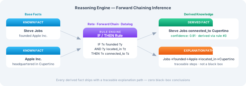
这张图就是 ReasoningPath 的可视化：起点是事实节点，中间是规则应用步，终点是结论；每条边都标注依据。监管者顺着图走一遍，"AI 为什么得出这个结论"就有了逐行可回放的答案。

五、装配位：解释器串起可信链路

把本章三节连起来看，reasoning 模块在管线中的完整出场顺序是：Rete/Reasoner 推出新事实 → Datalog/SPARQL 回答查询 → 溯因提假设、演绎做验证 → ExplanationGenerator 出具解释。解释对象与第 7 章的溯源层天然咬合：推理步引用的事实各有 PROV-O 档案（从哪个文档抽出来、谁抽取的），推理本身经 ReasoningEngineWithProvenance 包装后也会作为 Activity 记入溯源账本（reasoning_provenance.py，74 行——推理发生时间、前提数量、置信度一并归档）。于是第 6 章的 record_decision 引用一条推理结论时，"决策→推理→事实→原始文档"的完整解释链在图上全部可遍历——这就是"AI 拒贷必须说清为什么"的工程答案。

💡 装配要点：演绎与溯因共享 _parse_predicate/_unify 工具但方向相反——演绎从条件推结论（_find_matches 正向枚举绑定、_prove_backward 反向证定理），溯因从结论反查规则生成假设（四策略排序：simplicity/plausibility/consistency/coverage，默认 0.4/0.3/0.3 组合分）。ExplanationGenerator 的三分法要记牢：ReasoningStep 是原子、ReasoningPath 是序列、Justification 是带证据的裁决；detail_level 三档决定给监管看摘要还是全链。装配顺序：溯因出假设 → 演绎验证 → 解释器出报告，任何一步的产物都可继续流向下一段管线。

本节要点回顾

• 演绎：Premise/Conclusion/Proof/Argument 四件套；apply_logic 正向推结论（_find_matches 递归绑定，proof_steps 自带审计），prove_theorem/_prove_backward 反向证定理，validate_argument 出裁决。
• 溯因：Observation→Hypothesis→Explanation；_rule_explains_observation 用结论匹配观察、把条件反提为前提；simplicity=1/(1+条件数)，默认组合分 0.4/0.3/0.3；coverage/consistency 目前为占位常量。
• 数学差异：演绎 A→B 且 A ⊢ B 必然为真；溯因 B 观察到则猜 A，仅最佳解释，可错需验证。实践中溯因提假设、演绎验证。
• ExplanationGenerator：按 InferenceResult/Proof/AbductiveExplanation 分发；ReasoningStep（规则+输入+输出）→ ReasoningPath（起点/终点/总置信度）→ Justification（支持证据+解释文本）；detail_level 三档人类可读输出。
• 与第 7 章衔接：推理经 ReasoningEngineWithProvenance 记入 PROV-O 账本，决策→推理→事实→文档全链可遍历。

下一节：进入第 6 章压轴《决策智能》——01 ContextGraph 与 record_decision ★：4260 行的统一上下文图如何把每次 AI 决策变成图上可查的节点。