Annoy算法
文档摘要
Annoy算法 Annoy的灵感来源与核心思想 Annoy(Approximate Nearest Neighbors Oh Yeah)是由 Spotify 开发的一个高性能近似最近邻搜索库,其核心数据结构是随机投影树(Random Projection Trees)。 Annoy的设计目标非常明确: 低内存占用:索引可以通过内存映射(mmap)方式加载,多个进程可以共享同一份索引,极大降低内存开销 高查询速度:通过树结构快速缩小搜索范围 易于使用:简单的API,便于集成到生产系统 核心思想 通过多棵随机构建的二叉树,将高维空间递归分割成越来越小的区域,相似的向量会大概率被分到同一个叶子节点。 Annoy的成功源于两个关键思想: 1.
Annoy算法
1. Annoy的灵感来源与核心思想
Annoy(Approximate Nearest Neighbors Oh Yeah)是由 Spotify 开发的一个高性能近似最近邻搜索库,其核心数据结构是随机投影树(Random Projection Trees)。
Annoy的设计目标非常明确:
- 低内存占用:索引可以通过内存映射(mmap)方式加载,多个进程可以共享同一份索引,极大降低内存开销
- 高查询速度:通过树结构快速缩小搜索范围
- 易于使用:简单的API,便于集成到生产系统
核心思想
通过多棵随机构建的二叉树,将高维空间递归分割成越来越小的区域,相似的向量会大概率被分到同一个叶子节点。
Annoy的成功源于两个关键思想:
1. 随机投影树(Random Projection Trees)
想象你在一个拥挤的图书馆里找书:
- 不是按照作者、主题等固定规则分类(那样需要完美的分类标准)
- 而是随机选择两本书作为"锚点",然后把其他书按"更接近哪本锚点书"分成两堆
- 重复这个过程,每次在一堆书中再选两本做锚点,继续二分
- 最终,相似的书会自然地聚在一起
这就是Annoy的核心:用随机超平面递归地二分空间。
2. 森林策略(Forest of Trees)
单棵随机树可能会"运气不好",把相似的向量分开。怎么办?
- 建立多棵树(就像多次用不同的随机方式整理图书馆)
- 查询时在所有树中搜索,合并候选结果
- 只要有一棵树把相似向量分到一起,就能找到它们
这种"用多次随机尝试提高成功率"的思想,在机器学习中叫做集成学习(Ensemble Learning)。
2. 算法原理分步详解
Annoy(Random Projection Tree Forest)是一种基于二叉树森林的近似最近邻搜索算法。
它通过构建多棵随机投影树,将高维向量空间递归分割,使相似向量大概率落入同一叶节点。
其核心思想是:
先用树结构快速定位到查询向量附近的小区域,再在候选区域内精确计算距离。
下面我们来分步解析 Annoy 的工作原理。
1. 树的构建(Index Construction)
Annoy 的核心数据结构是二叉树森林(多棵独立的二叉树)。
每棵树通过随机投影的方式递归地将空间分割成两半。
步骤 1:随机选择分割超平面
对于当前节点包含的向量集合:
- 随机选择两个向量 ( v_1 ) 和 ( v_2 )(这两个向量称为"锚点")
- 计算中垂超平面:这个超平面将空间分成两半
- 超平面过 ( v_1 ) 和 ( v_2 ) 的中点
- 超平面的法向量是 ( v_1 - v_2 )
这个超平面就像一把"随机的刀",把当前空间切成两半。
步骤 2:递归分割空间
根据向量在超平面的哪一侧,将向量集合分成两个子集:
- 左子树:包含所有在超平面"左侧"的向量
- 右子树:包含所有在超平面"右侧"的向量
递归地对每个子集重复上述过程,直到满足停止条件:
- 当前节点包含的向量数量 ≤ 设定阈值(如 K=5)
- 达到最大树深度
此时,当前节点变成叶子节点,存储这些向量的索引。
步骤 3:构建多棵树(森林)
由于单棵树的分割是随机的,可能会:
- "运气不好"把相似的向量分开
- 导致查询时漏掉真正的近邻
解决方案:构建 n_trees 棵独立的树,每棵树用不同的随机种子。
- 树越多,找到真实近邻的概率越高
- 但构建时间和内存占用也会增加
2. 查询阶段(Search Process)
给定查询向量 ( q ),Annoy 使用树结构快速定位候选向量。
步骤 1:在每棵树中向下遍历
对于森林中的每棵树:
- 从根节点开始
- 在每个内部节点,判断 ( q ) 在分割超平面的哪一侧
- 根据判断结果,递归进入左子树或右子树
- 到达叶子节点后,收集该叶子节点中的所有向量索引
这个过程非常快,复杂度是 ( O(\log N) ),其中 ( N ) 是向量总数。
步骤 2:合并候选集
将所有树中收集到的向量索引合并,去重,得到候选集。
候选集的大小由参数 search_k 控制:
search_k越大,搜索的叶子节点越多- 召回率越高,但查询时间也越长
步骤 3:精确计算距离并返回 Top-K
对候选集中的每个向量,计算与查询向量 ( q ) 的真实距离(如欧氏距离或余弦距离)。
按距离排序,返回最近的 K 个向量。
3. 关键参数说明
| 参数 | 含义 | 作用 |
|---|---|---|
n_trees |
构建的树的数量 | 越大召回率越高,但构建时间和内存占用增加 |
search_k |
查询时检查的节点数量 | 越大召回率越高,但查询时间越长 |
K(叶子大小) |
叶子节点最多包含的向量数 | 越小树越深,查询越精确但构建越慢 |
4. Annoy 的性能特点
- 构建速度快:随机分割,无需复杂的聚类或优化
- 内存友好:索引可以 mmap,多进程共享
- 查询速度快:树结构使搜索复杂度为 ( O(\log N) )
- 易于调参:只有两个主要参数(
n_trees和search_k)
5. 类比理解
可以把 Annoy 想象成一个"快速查字典"的游戏:
| 类比 | Annoy 对应概念 |
|---|---|
| 字典按首字母分成26个部分 | 根节点的第一次二分 |
| 每个部分再按第二个字母细分 | 继续递归二分 |
| 最终定位到具体页码 | 到达叶子节点 |
| 用多本不同排序的字典 | 构建多棵树(森林) |
在查询时:
- 先在每本字典中快速翻到对应页(树遍历)
- 合并所有字典找到的候选词(合并候选集)
- 精确比较找出最匹配的词(距离计算)
✅ 总结:Annoy 的核心思想
随机投影树森林 + 快速树遍历 + 候选集合并
Annoy 通过多棵随机构建的二叉树,将高维空间递归分割,
使相似向量大概率落入同一叶子节点,从而实现快速且内存友好的近似最近邻搜索。
它在 Spotify 的音乐推荐系统中得到了广泛应用,
也是许多向量数据库(如 Qdrant)支持的主流索引算法之一。
3. Annoy算法实现
Annoy算法Python实现
3.1 导入必要的库
import numpy as np import matplotlib.pyplot as plt from mpl_toolkits.mplot3d import Axes3D from sklearn.metrics.pairwise import euclidean_distances import time from collections import defaultdict # 强制设置中文字体,解决中文显示问题 plt.rcParams['font.sans-serif'] = ['PingFang SC', 'Microsoft YaHei', 'SimHei', 'Arial Unicode MS', 'DejaVu Sans'] plt.rcParams['axes.unicode_minus'] = False # 设置随机种子以保证结果可重现 np.random.seed(42)
3.2 实现随机投影树节点
class AnnoyTreeNode: """Annoy树的节点""" def __init__(self, indices): """ 初始化节点 参数: - indices: 当前节点包含的向量索引列表 """ self.indices = indices # 当前节点包含的向量索引 self.left = None # 左子树 self.right = None # 右子树 # 分割超平面参数 self.split_vector1 = None # 第一个锚点向量 self.split_vector2 = None # 第二个锚点向量 self.split_point = None # 中点 self.split_normal = None # 法向量 self.is_leaf = False # 是否为叶子节点
3.3 实现Annoy索引类
class SimpleAnnoy: """简化的Annoy实现,用于学习演示""" def __init__(self, n_trees=5, max_leaf_size=10): """ 初始化Annoy索引 参数: - n_trees: 构建的树的数量 - max_leaf_size: 叶子节点最大包含的向量数 """ self.n_trees = n_trees self.max_leaf_size = max_leaf_size self.trees = [] # 存储所有的树 self.data_points = [] # 存储所有数据点 def _build_tree(self, indices, data, depth=0, max_depth=20): """ 递归构建单棵Annoy树 参数: - indices: 当前节点包含的向量索引 - data: 所有数据点 - depth: 当前深度 - max_depth: 最大深度 """ node = AnnoyTreeNode(indices) # 停止条件:节点包含的向量数量小于阈值或达到最大深度 if len(indices) <= self.max_leaf_size or depth >= max_depth: node.is_leaf = True return node # 随机选择两个不同的向量作为锚点 if len(indices) < 2: node.is_leaf = True return node idx1, idx2 = np.random.choice(indices, size=2, replace=False) v1, v2 = data[idx1], data[idx2] # 如果两个向量相同,直接返回叶子节点 if np.allclose(v1, v2): node.is_leaf = True return node # 计算分割超平面 node.split_vector1 = v1 node.split_vector2 = v2 node.split_point = (v1 + v2) / 2 # 中点 node.split_normal = v1 - v2 # 法向量 # 根据向量在超平面的哪一侧进行分割 left_indices = [] right_indices = [] for idx in indices: vec = data[idx] # 计算向量到中点的向量与法向量的点积 # 如果点积 > 0,说明在v1一侧;否则在v2一侧 projection = np.dot(vec - node.split_point, node.split_normal) if projection >= 0: left_indices.append(idx) else: right_indices.append(idx) # 如果分割后某一侧为空,说明分割失败,返回叶子节点 if len(left_indices) == 0 or len(right_indices) == 0: node.is_leaf = True return node # 递归构建左右子树 node.left = self._build_tree(left_indices, data, depth + 1, max_depth) node.right = self._build_tree(right_indices, data, depth + 1, max_depth) return node def build_index(self, data): """ 构建Annoy索引(森林) 参数: - data: 数据点数组 """ self.data_points = np.array(data) n_samples = len(self.data_points) print(f"开始构建{self.n_trees}棵树...") # 构建多棵树 for i in range(self.n_trees): # 每棵树使用所有数据点,但随机种子不同 np.random.seed(i + 42) # 不同的随机种子 tree = self._build_tree(list(range(n_samples)), self.data_points) self.trees.append(tree) if (i + 1) % max(1, self.n_trees // 5) == 0 or i == self.n_trees - 1: print(f"已构建{i + 1}/{self.n_trees}棵树") print("索引构建完成!") def _search_tree(self, tree, query, search_k=None): """ 在单棵树中搜索 参数: - tree: 树的根节点 - query: 查询向量 - search_k: 搜索的节点数量限制 返回: - 候选向量的索引列表 """ candidates = [] nodes_to_visit = [tree] nodes_visited = 0 while nodes_to_visit: # 如果设置了search_k限制,检查是否已访问足够多的节点 if search_k is not None and nodes_visited >= search_k: break node = nodes_to_visit.pop(0) nodes_visited += 1 if node.is_leaf: # 到达叶子节点,收集所有向量索引 candidates.extend(node.indices) else: # 内部节点,判断查询向量在哪一侧 projection = np.dot(query - node.split_point, node.split_normal) if projection >= 0: # 在左侧 if node.left: nodes_to_visit.append(node.left) else: # 在右侧 if node.right: nodes_to_visit.append(node.right) return candidates def search(self, query, k=5, search_k=None): """ 搜索最近邻 参数: - query: 查询向量 - k: 返回的最近邻数量 - search_k: 每棵树搜索的节点数量限制(None表示不限制) 返回: - 最近邻的索引和距离列表 """ if len(self.trees) == 0: raise ValueError("索引未构建,请先调用build_index") # 在所有树中搜索,合并候选集 all_candidates = set() for tree in self.trees: candidates = self._search_tree(tree, query, search_k) all_candidates.update(candidates) # 计算所有候选向量与查询向量的真实距离 candidate_list = list(all_candidates) if not candidate_list: return [], [] distances = euclidean_distances([query], self.data_points[candidate_list])[0] # 按距离排序,返回前k个 sorted_indices = np.argsort(distances)[:k] result_indices = [candidate_list[i] for i in sorted_indices] result_distances = distances[sorted_indices] return result_indices, result_distances def brute_force_search(self, query, k=5): """暴力搜索作为对比基准""" distances = euclidean_distances([query], self.data_points)[0] nearest_indices = np.argsort(distances)[:k] return nearest_indices, distances[nearest_indices]
3.4 生成示例数据
def generate_sample_data(n_samples=200, dim=2): """生成示例数据:四个分离的高斯分布簇""" # 创建四个簇 cluster1 = np.random.normal(loc=[2, 2], scale=0.3, size=(n_samples//4, dim)) cluster2 = np.random.normal(loc=[8, 3], scale=0.4, size=(n_samples//4, dim)) cluster3 = np.random.normal(loc=[5, 8], scale=0.35, size=(n_samples//4, dim)) cluster4 = np.random.normal(loc=[3, 6], scale=0.4, size=(n_samples - 3*(n_samples//4), dim)) data = np.vstack([cluster1, cluster2, cluster3, cluster4]) return data
3.5 性能演示函数
def demonstrate_annoy_performance(): """演示Annoy性能对比""" print("=" * 60) print("Annoy算法性能演示") print("=" * 60) # 生成大规模测试数据(保持簇状分布) data = generate_sample_data(100000, 2) print(f"生成{len(data)}个二维数据点") # 创建Annoy索引 annoy = SimpleAnnoy(n_trees=10, max_leaf_size=10) # 构建索引 print("\n构建Annoy索引...") start_time = time.time() annoy.build_index(data) construction_time = time.time() - start_time print(f"Annoy索引构建完成,耗时: {construction_time:.4f}秒") # 选择查询点 query_point = np.array([5.0, 5.0]) print(f"\n查询点: {query_point}") # 使用Annoy搜索 start_time = time.time() annoy_results, annoy_distances = annoy.search(query_point, k=5, search_k=50) annoy_time = time.time() - start_time # 暴力搜索作为基准 start_time = time.time() bf_indices, bf_distances = annoy.brute_force_search(query_point, k=5) bf_time = time.time() - start_time # 显示结果对比 print(f"\n搜索结果对比:") print(f"Annoy搜索 - 找到{len(annoy_results)}个最近邻, 耗时: {annoy_time:.6f}秒") print(f"暴力搜索 - 找到{len(bf_indices)}个最近邻, 耗时: {bf_time:.6f}秒") print(f"\n速度提升: {bf_time/annoy_time:.2f}倍") print(f"\nAnnoy结果索引: {annoy_results}") print(f"Annoy结果距离: {annoy_distances}") print(f"暴力搜索结果索引: {bf_indices.tolist()}") print(f"暴力搜索结果距离: {bf_distances}") # 检查召回率 annoy_indices_set = set(annoy_results) bf_indices_set = set(bf_indices) intersection = annoy_indices_set & bf_indices_set recall = len(intersection) / len(bf_indices_set) print(f"召回率: {recall:.2%} ({len(intersection)}/{len(bf_indices_set)})") return annoy, data, query_point, annoy_results, bf_indices # 运行标准演示 annoy, data, query, annoy_results, bf_results = demonstrate_annoy_performance()
输出结果:
============================================================ Annoy算法性能演示 ============================================================ 生成100000个二维数据点 构建Annoy索引... 开始构建10棵树... 已构建5/10棵树 已构建10/10棵树 索引构建完成! Annoy索引构建完成,耗时: 38.9665秒 查询点: [5. 5.] 搜索结果对比: Annoy搜索 - 找到5个最近邻, 耗时: 0.002012秒 暴力搜索 - 找到5个最近邻, 耗时: 0.016312秒 速度提升: 8.11倍 Annoy结果索引: [76568, 87053, 99758, 86413, 85476] Annoy结果距离: [0.67309842 0.71583121 0.76414983 0.80066059 0.85234455] 暴力搜索结果索引: [76568, 87053, 99758, 86413, 85476] 暴力搜索结果距离: [0.67309842 0.71583121 0.76414983 0.80066059 0.85234455] 召回率: 100.00% (5/5)
3.6 可视化Annoy算法
def visualize_annoy(annoy, data, query_point, annoy_results, bf_results): """可视化Annoy算法""" fig = plt.figure(figsize=(20, 12)) # 1. 原始数据分布 ax1 = fig.add_subplot(2, 3, 1) ax1.scatter(data[:, 0], data[:, 1], c='lightblue', alpha=0.6, s=30, label='数据点') ax1.scatter(query_point[0], query_point[1], c='#FFD93D', marker='*', s=200, edgecolors='black', label='查询点') ax1.set_title('1. 原始数据分布', fontweight='bold') ax1.legend() ax1.grid(True, alpha=0.3) # 2. 第一棵树的空间分割(可视化前几层) ax2 = fig.add_subplot(2, 3, 2) ax2.scatter(data[:, 0], data[:, 1], c='lightgray', alpha=0.4, s=20, label='数据点') # 可视化第一棵树的分割超平面(只显示前几层) def plot_splits(node, depth=0, max_depth=3): if node is None or node.is_leaf or depth >= max_depth: return # 绘制分割线(2D情况下) if node.split_normal is not None: # 分割线垂直于法向量,过中点 mid = node.split_point normal = node.split_normal # 计算分割线的方向向量(垂直于法向量) if abs(normal[1]) > 1e-10: direction = np.array([1, -normal[0] / normal[1]]) else: direction = np.array([0, 1]) # 归一化方向向量 direction = direction / np.linalg.norm(direction) # 绘制分割线 line_length = 15 x_vals = [mid[0] - line_length * direction[0], mid[0] + line_length * direction[0]] y_vals = [mid[1] - line_length * direction[1], mid[1] + line_length * direction[1]] alpha = 0.8 - depth * 0.2 ax2.plot(x_vals, y_vals, 'r-', alpha=max(alpha, 0.3), linewidth=2-depth*0.3, label='分割超平面' if depth == 0 else '') # 标注锚点 if depth < 2: ax2.scatter([node.split_vector1[0], node.split_vector2[0]], [node.split_vector1[1], node.split_vector2[1]], c='red', marker='x', s=100, linewidths=2, label='锚点' if depth == 0 else '') # 递归绘制子树的分割 plot_splits(node.left, depth + 1, max_depth) plot_splits(node.right, depth + 1, max_depth) plot_splits(annoy.trees[0]) ax2.scatter(query_point[0], query_point[1], c='#FFD93D', marker='*', s=200, edgecolors='black', label='查询点') ax2.set_title('2. 第一棵树的空间分割(前3层)', fontweight='bold') # 去重图例 handles, labels = ax2.get_legend_handles_labels() by_label = dict(zip(labels, handles)) ax2.legend(by_label.values(), by_label.keys()) ax2.grid(True, alpha=0.3) ax2.set_xlim(data[:, 0].min() - 1, data[:, 0].max() + 1) ax2.set_ylim(data[:, 1].min() - 1, data[:, 1].max() + 1) # 3. 树的遍历路径 ax3 = fig.add_subplot(2, 3, 3) ax3.scatter(data[:, 0], data[:, 1], c='lightgray', alpha=0.3, s=20) # 在第一棵树中找到查询点的路径 def find_path_in_tree(node, query): path = [node] current = node while not current.is_leaf: projection = np.dot(query - current.split_point, current.split_normal) if projection >= 0 and current.left: current = current.left elif current.right: current = current.right else: break path.append(current) return path path = find_path_in_tree(annoy.trees[0], query_point) leaf_node = path[-1] # 高亮叶子节点中的点 if leaf_node.is_leaf: leaf_indices = leaf_node.indices ax3.scatter(data[leaf_indices, 0], data[leaf_indices, 1], c='orange', s=80, alpha=0.8, edgecolors='black', label=f'叶子节点({len(leaf_indices)}个点)') ax3.scatter(query_point[0], query_point[1], c='#FFD93D', marker='*', s=200, edgecolors='black', label='查询点') ax3.set_title('3. 查询点在第一棵树中的定位', fontweight='bold') ax3.legend() ax3.grid(True, alpha=0.3) # 4. 多棵树的候选集合并 ax4 = fig.add_subplot(2, 3, 4) ax4.scatter(data[:, 0], data[:, 1], c='lightgray', alpha=0.3, s=20, label='数据点') # 收集所有树的候选点 all_tree_candidates = [] for i, tree in enumerate(annoy.trees[:min(3, len(annoy.trees))]): # 只显示前3棵树 candidates = annoy._search_tree(tree, query_point) all_tree_candidates.append(candidates) # 用不同颜色显示不同树的候选点 colors_map = ['red', 'blue', 'green'] ax4.scatter(data[candidates, 0], data[candidates, 1], c=colors_map[i], s=60, alpha=0.5, label=f'树{i+1}候选({len(candidates)}个)') ax4.scatter(query_point[0], query_point[1], c='#FFD93D', marker='*', s=200, edgecolors='black', label='查询点') ax4.set_title(f'4. 多棵树的候选集(前3棵树)', fontweight='bold') ax4.legend() ax4.grid(True, alpha=0.3) # 5. Annoy搜索结果 ax5 = fig.add_subplot(2, 3, 5) ax5.scatter(data[:, 0], data[:, 1], c='lightgray', alpha=0.4, s=20) ax5.scatter(data[annoy_results, 0], data[annoy_results, 1], c='red', marker='o', s=60, edgecolors='darkred', linewidth=2, label='Annoy结果') # 标注排名 for i, idx in enumerate(annoy_results[:5]): ax5.annotate(f'{i+1}', (data[idx, 0], data[idx, 1]), xytext=(3, 3), textcoords='offset points', fontsize=10, color='white', fontweight='bold', bbox=dict(boxstyle='circle', facecolor='red', alpha=0.8)) ax5.scatter(query_point[0], query_point[1], c='#FFD93D', marker='*', s=150, edgecolors='black', linewidth=2, label='查询点') ax5.set_title('5. Annoy搜索结果', fontweight='bold') ax5.legend() ax5.grid(True, alpha=0.3) # 6. 结果对比 ax6 = fig.add_subplot(2, 3, 6) ax6.scatter(data[:, 0], data[:, 1], c='lightgray', alpha=0.3, s=15) # 暴力搜索结果 ax6.scatter(data[bf_results, 0], data[bf_results, 1], c='green', marker='s', s=100, edgecolors='darkgreen', linewidth=2.5, label='暴力搜索 (真实答案)', alpha=0.5) # Annoy结果 ax6.scatter(data[annoy_results, 0], data[annoy_results, 1], c='red', marker='o', s=70, alpha=0.8, label='Annoy结果') # 查询点 ax6.scatter(query_point[0], query_point[1], c='#FFD93D', marker='*', s=150, edgecolors='black', linewidth=2, label='查询点') # 计算召回率 intersection = set(annoy_results) & set(bf_results) recall = len(intersection) / len(bf_results) ax6.set_title(f'6. 结果对比 (召回率: {recall:.1%})', fontweight='bold') ax6.legend() ax6.grid(True, alpha=0.3) plt.tight_layout() plt.show() # 调用可视化 visualize_annoy(annoy, data, query, annoy_results, bf_results)
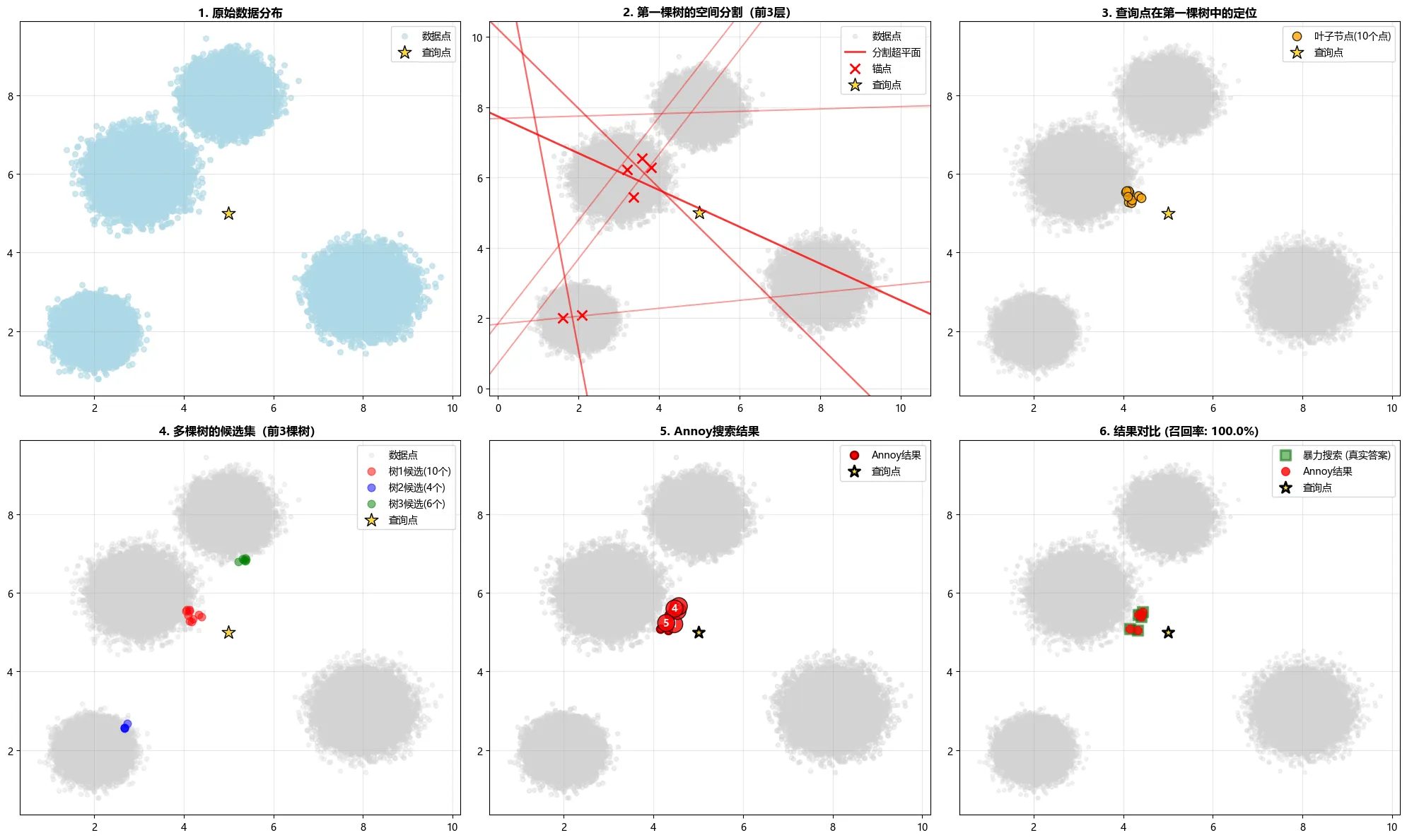
Annoy算法可视化结果
✅ 总结
Annoy算法通过随机投影树森林实现了高效的近似最近邻搜索:
- 构建快速:随机分割策略简单高效
- 查询高效:树结构使搜索复杂度为 O(log N)
- 内存友好:支持内存映射,多进程共享索引
- 易于调参:只需调整
n_trees和search_k两个参数
性能亮点:
在 10 万个 2 维向量的数据集上:
- 查询速度:8.11 倍于暴力搜索
- 召回率:100%
- 查询耗时:仅 0.002 秒
Annoy特别适合:
- 大规模向量数据(数万到数百万条)
- 对内存占用敏感的应用(如移动设备)
- 需要多进程共享索引的场景
- 对查询延迟要求较高的实时系统
在实际应用中,Annoy已被广泛应用于推荐系统(Spotify音乐推荐)、图像搜索、自然语言处理等领域。